# Histogram of 100000 random values from a sample of 100 with probability of 0.5
hist(rbinom(100000, size = 100, prob = 0.5))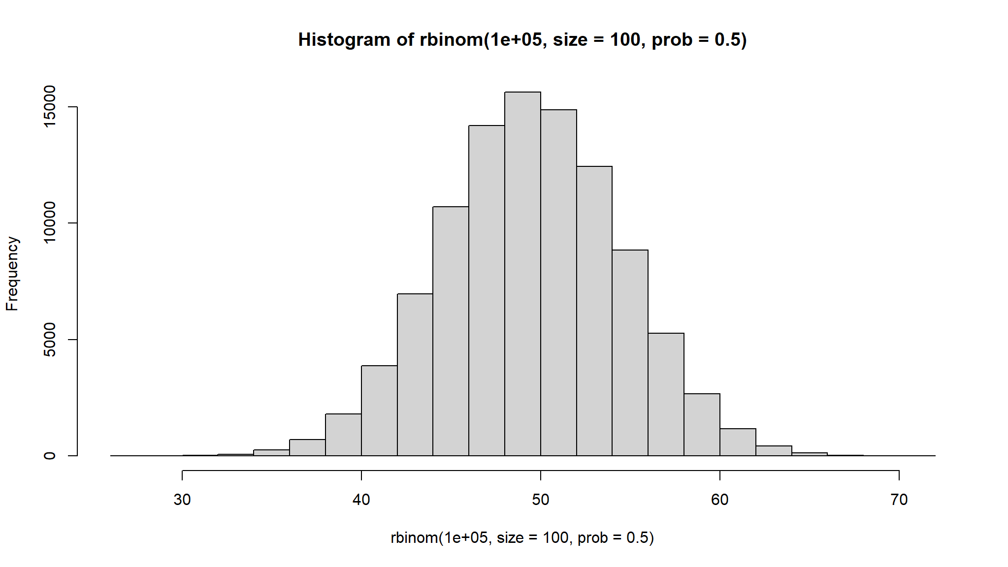
If you feel you do not need to brush up on these theories, you can jump right into [Descriptive Statistics]
\[\begin{equation} \begin{split} A= \left[\begin{array} {cc} a_{11} & a_{12} \\ a_{21} & a_{22} \\ \end{array} \right] \end{split} \end{equation}\]
\[\begin{equation} \begin{split} A' = \left[\begin{array} {cc} a_{11} & a_{21} \\ a_{12} & a_{22} \\ \end{array} \right] \end{split} \end{equation}\]
\[ \mathbf{(ABC)'=C'B'A'} \\ \mathbf{A(B+C)= AB + AC} \\ \mathbf{AB \neq BA} \\ \mathbf{(A')'=A} \\ \mathbf{(A+B)' = A' + B'} \\ \mathbf{(AB)' = B'A'} \\ \mathbf{(AB)^{-1}= B^{-1}A^{-1}} \\ \mathbf{A+B = B +A} \\ \mathbf{AA^{-1} = I } \]
If A has an inverse, it is called invertible. If A is not invertible it is called singular.
\[\begin{equation} \begin{split} \mathbf{A} &= \left(\begin{array} {ccc} a_{11} & a_{12} & a_{13} \\ a_{21} & a_{22} & a_{23} \\ \end{array}\right) \left(\begin{array} {ccc} b_{11} & b_{12} & b_{13} \\ b_{21} & b_{22} & b_{23} \\ b_{31} & b_{32} & b_{33} \\ \end{array}\right) \\ &= \left(\begin{array} {ccc} a_{11}b_{11}+a_{12}b_{21}+a_{13}b_{31} & \sum_{i=1}^{3}a_{1i}b_{i2} & \sum_{i=1}^{3}a_{1i}b_{i3} \\ \sum_{i=1}^{3}a_{2i}b_{i1} & \sum_{i=1}^{3}a_{2i}b_{i2} & \sum_{i=1}^{3}a_{2i}b_{i3} \\ \end{array}\right) \end{split} \end{equation}\]
Let \(\mathbf{a}\) be a 3 x 1 vector, then the quadratic form is
\[ \mathbf{a'Ba} = \sum_{i=1}^{3}\sum_{i=1}^{3}a_i b_{ij} a_{j} \]
Length of a vector
Let \(\mathbf{a}\) be a vector, \(||\mathbf{a}||\) (the 2-norm of the vector) is the length of vector \(\mathbf{a}\), is the square root of the inner product of the vector with itself:
\[ ||\mathbf{a}|| = \sqrt{\mathbf{a'a}} \]
For a n x k matrix A and k x k matrix B
In scalar, a = 0 then 1/a does not exist. In matrix, a matrix is invertible when it’s a non-zero matrix.
A non-singular square matrix A is invertible if there exists a non-singular square matrix B such that, \[AB=I\] Then \(A^{-1}=B\). For a 2x2 matrix,
\[ A = \left(\begin{array}{cc} a & b \\ c & d \\ \end{array} \right) \]
\[ A^{-1}= \frac{1}{ad-bc} \left(\begin{array}{cc} d & -b \\ -c & a \\ \end{array} \right) \]
For the partition matrix,
\[\begin{equation} \begin{split} \left[\begin{array} {cc} A & B \\ C & D \\ \end{array} \right]^{-1} = \left[\begin{array} {cc} \mathbf{(A-BD^{-1}C)^{-1}} & \mathbf{-(A-BD^{-1}C)^{-1}BD^-1}\\ \mathbf{-DC(A-BD^{-1}C)^{-1}} & \mathbf{D^{-1}+D^{-1}C(A-BD^{-1}C)^{-1}BD^{-1}}\ \\ \end{array} \right] \end{split} \end{equation}\]
Properties for a non-singular square matrix
A symmetric square k x k matrix, \(\mathbf{A}\), is Positive Semi-Definite if for any non-zero k x 1 vector \(\mathbf{x}\), \[\mathbf{x'Ax \geq 0 }\]
A symmetric square k x k matrix, \(\mathbf{A}\), is Negative Semi-Definite if for any non-zero k x 1 vector \(\mathbf{x}\) \[\mathbf{x'Ax \leq 0 }\]
\(\mathbf{A}\) is indefinite if it is neither positive semi-definite or negative semi-definite.
The identity matrix is positive definite
Example Let \(\mathbf{x} =(x_1 x_2)'\), then for a 2 x 2 identity matrix,
\[\begin{equation} \begin{split} \mathbf{x'Ix} &= (x_1 x_2) \left(\begin{array} {cc} 1 & 0 \\ 0 & 1 \\ \end{array} \right) \left(\begin{array}{c} x_1 \\ x_2 \\ \end{array} \right) \\ &= (x_1 x_2) \left(\begin{array} {c} x_1 \\ x_2 \\ \end{array} \right) \\ &= x_1^2 + x_2^2 >0 \end{split} \end{equation}\]
Definiteness gives us the ability to compare matrices \(\mathbf{A-B}\) is PSD This property also helps us show efficiency (which variance covariance matrix of one estimator is smaller than another)
Properties
Note
Example:
\[ \left[ \begin{array} {cc} -1 & 0 \\ 0 & 10 \\ \end{array} \right] \]
\[ \left[ \begin{array} {cc} 0 & 1 \\ 0 & 0 \\ \end{array} \right] \]
\[ \left[ \begin{array} {cc} 1 & 0 \\ 0 & 1 \\ \end{array} \right] \]
\[ \left[ \begin{array} {cc} 0 & 0 \\ 0 & 1 \\ \end{array} \right] \]
\(y=f(x_1,x_2,...,x_k)=f(x)\) where x is a 1 x k row vector. The Gradient (first order derivative with respect to a vector) is,
\[ \frac{\partial{f(x)}}{\partial{x}}= \left(\begin{array}{c} \frac{\partial{f(x)}}{\partial{x_1}} \\ \frac{\partial{f(x)}}{\partial{x_2}} \\ ... \\ \frac{\partial{f(x)}}{\partial{x_k}} \end{array} \right) \]
The Hessian (second order derivative with respect to a vector) is,
\[ \frac{\partial^2{f(x)}}{\partial{x}\partial{x'}}= \left(\begin{array} {cccc} \frac{\partial^2{f(x)}}{\partial{x_1}\partial{x_1}} & \frac{\partial^2{f(x)}}{\partial{x_1}\partial{x_2}} & ... & \frac{\partial^2{f(x)}}{\partial{x_1}\partial{x_k}} \\ \frac{\partial^2{f(x)}}{\partial{x_1}\partial{x_2}} & \frac{\partial^2{f(x)}}{\partial{x_2}\partial{x_2}} & ... & \frac{\partial^2{f(x)}}{\partial{x_2}\partial{x_k}} \\ ... & ...& & ...\\ \frac{\partial^2{f(x)}}{\partial{x_k}\partial{x_1}} & \frac{\partial^2{f(x)}}{\partial{x_k}\partial{x_2}} & ... & \frac{\partial^2{f(x)}}{\partial{x_k}\partial{x_k}} \end{array} \right) \]
Define the derivative of \(f(\mathbf{X})\) with respect to \(\mathbf{X}_{(n \times p)}\) as the matrix
\[ \frac{\partial f(\mathbf{X})}{\partial \mathbf{X}} = (\frac{\partial f(\mathbf{X})}{\partial x_{ij}}) \]
Define \(\mathbf{a}\) to be a vector and \(\mathbf{A}\) to be a matrix which does not depend upon \(\mathbf{y}\). Then
\[ \frac{\partial \mathbf{a'y}}{\partial \mathbf{y}} = \mathbf{a} \]
\[ \frac{\partial \mathbf{y'y}}{\partial \mathbf{y}} = 2\mathbf{y} \]
\[ \frac{\partial \mathbf{y'Ay}}{\partial \mathbf{y}} = \mathbf{(A + A')y} \]
If \(\mathbf{X}\) is a symmetric matrix then
\[ \frac{\partial |\mathbf{X}|}{\partial x_{ij}} = \begin{cases} X_{ii}, i = j \\ X_ij, i \neq j \end{cases} \] where \(X_{ij}\) is the (i,j)th cofactor of \(\mathbf{X}\)
If \(\mathbf{X}\) is symmetric and \(\mathbf{A}\) is a matrix which does not depend upon \(\mathbf{X}\) then
\[ \frac{\partial tr \mathbf{XA}}{\partial \mathbf{X}} = \mathbf{A} + \mathbf{A}' - diag(\mathbf{A}) \]
If \(\mathbf{X}\) is symmetric and we let \(\mathbf{J}_{ij}\) be a matrix which has a 1 in the (i,j)th position and 0s elsewhere, then
\[ \frac{\partial \mathbf{X}6{-1}}{\partial x_{ij}} = \begin{cases} - \mathbf{X}^{-1}\mathbf{J}_{ii} \mathbf{X}^{-1} , i = j \\ - \mathbf{X}^{-1}(\mathbf{J}_{ij} + \mathbf{J}_{ji}) \mathbf{X}^{-1} , i \neq j \end{cases} \]
| Scalar Optimization | Vector Optimization | |
|---|---|---|
| First Order Condition | \[\frac{\partial{f(x_0)}}{\partial{x}}=0\] | \[\frac{\partial{f(x_0)}}{\partial{x}}=\left(\begin{array}{c}0 \\ .\\ .\\ .\\ 0\end{array}\right)\] |
|
Second Order Condition Convex \(\rightarrow\) Min |
\[\frac{\partial^2{f(x_0)}}{\partial{x^2}} > 0\] | \[\frac{\partial^2{f(x_0)}}{\partial{xx'}}>0\] |
| Concave \(\rightarrow\) Max | \[\frac{\partial^2{f(x_0)}}{\partial{x^2}} < 0\] | \[\frac{\partial^2{f(x_0)}}{\partial{xx'}}<0\] |
Conditional Probability
\[ P[A|B]=\frac{A \cap B}{P[B]} \]
Independent Events Two events A and B are independent if and only if:
A finite collection of events \(A_1, A_2, ..., A_n\) is independent if and only if any subcollection is independent.
Multiplication Rule \(P[A \cap B] = P[A|B]P[B] = P[B|A]P[A]\)
Bayes’ Theorem Let \(A_1, A_2, ..., A_n\) be a collection of mutually exclusive events whose union is S.
Let b be an event such that \(P[B]\neq0\)
Then for any of the events \(A_j\), j = 1,2,…,n
\[ P[A_|B]=\frac{P[B|A_j]P[A_j]}{\sum_{i=1}^{n}P[B|A_j]P[A_i]} \]
Jensen’s Inequality
\(E(Y)=E(E(Y|X))\)
Independence
Mean Independence (implied by independence)
Uncorrelated (implied by independence and mean independence)
\[ Strongest \\ \downarrow \\ Independence \\ \downarrow \\ Mean Independence \\ \downarrow \\ Uncorrelated \\ \downarrow \\ Weakest\\ \]
Let \(X_1, X_2,...,X_n\) be a random sample of size n from a distribution (not necessarily normal) X with mean \(\mu\) and variance \(\sigma^2\). then for large n (\(n \ge 25\)),
\(\bar{X}\) is approximately normal with with mean \(\mu_{\bar{X}}=\mu\) and variance \(\sigma^2_{\bar{X}} = Var(\bar{X})= \frac{\sigma^2}{n}\)
\(\hat{p}\)is approximately normal with \(\mu_{\hat{p}} = p, \sigma^2_{\hat{p}} = \frac{p(1-p)}{n}\)
\(\hat{p_1} - \hat{p_2}\) is approximately normal with \(\mu_{\hat{p_1} - \hat{p_2}} = p_1 - p_2, \sigma^2_{\hat{p_1} - \hat{p_2}}=\frac{p_1(1-p)}{n_1} + \frac{p_2(1-p)}{n_2}\)
\(\bar{X_1} - \bar{X_2}\) is approximately normal with \(\mu_{\bar{X_1} - \bar{X_2}} = \mu_1 - \mu_2, \sigma^2_{\bar{X_1} - \bar{X_2}} = \frac{\sigma^2_1}{n_1}+\frac{\sigma^2_2}{n_2}\)
The following random variables are approximately standard normal:
If \(\{x_i\}_{i=1}^{n}\) is an iid random sample from a probability distribution with finite mean \(\mu\) and finite variance \(\sigma^2\) then the sample mean \(\bar{x}=n^{-1}\sum_{i=1}^{n}x_i\) scaled by \(\sqrt{n}\) has the following limiting distribution
\[ \sqrt{n}(\bar{x}-\mu) \to^d N(0,\sigma^2) \]
or if we were to standardize the sample mean,
\[ \frac{\sqrt{n}(\bar{x}-\mu)}{\sigma} \to^d N(0,1) \]
\[ Avar(\sqrt{n}(\bar{x}-\mu)) = \sigma^2 \\ \lim_{n \to \infty} Var(\sqrt{n}(\bar{x}-\mu)) = \sigma^2 \\ Avar(.) \neq lim_{n \to \infty} Var(.) \]
| Discrete Variable | Continuous Variable | |
|---|---|---|
| Definition | A random variable is discrete if it can assume at most a finite or countably infinite number of possible values | A random variable is continuous if it can assume any value in some interval or intervals of real numbers and the probability that it assumes any specific value is 0 |
| Density Function | A function f is called a density for X if: (1) \(f(x) \ge 0\) (2) \(\sum_{all~x}f(x)=1\) (3) \(f(x)=P(X=x)\) for x real |
A function f is called a density for X if: (1) \(f(x) \ge 0\) for x real (2) \(\int_{-\infty}^{\infty} f(x) \; dx=1\) (3) \(P[a \le X \le] =\int_{a}^{b} f(x) \; dx\) for a and b real |
|
Cumulative Distribution Function for x real |
\(F(x)=P[X \le x]\) | \(F(x)=P[X \le x]=\int_{-\infty}^{\infty}f(t)dt\) |
| \(E[H(X)]\) | \(\sum_{all ~x}H(x)f(x)\) | \(\int_{-\infty}^{\infty}H(x)f(x)\) |
| \(\mu=E[X]\) | \(\sum_{all ~ x}xf(x)\) | \(\int_{-\infty}^{\infty}xf(x)\) |
|
Ordinary Moments the kth ordinary moment for variable X is defined as: \(E[X^k]\) |
\(\sum_{all ~ x \in X}(x^kf(x))\) | \(\int_{-\infty}^{\infty}(x^kf(x))\) |
|
Moment generating function (mgf) \(m_X(t)=E[e^{tX}]\) |
\(\sum_{all ~ x \in X}(e^{tx}f(x))\) | \(\int_{-\infty}^{\infty}(e^{tx}f(x)dx)\) |
Expected Value Properties:
Expected Variance Properties:
Standard deviation \(\sigma=\sqrt(\sigma^2)=\sqrt(Var X)\)
Suppose \(y_1,...,y_p\) are possibly correlated random variables with means \(\mu_1,...,\mu_p\). then
\[ \mathbf{y} = (y_1,...,y_p)' \\ E(\mathbf{y}) = (\mu_1,...,\mu_p)' = \mathbf{\mu} \]
Let \(\sigma_{ij} = cov(y_i,y_j)\) for \(i,j = 1,..,p\).
Define
\[ \mathbf{\Sigma} = (\sigma_{ij}) = \left(\begin{array} {rrrr} \sigma_{11} & \sigma_{12} & ... & \sigma_{1p} \\ \sigma_{21} & \sigma_{22} & ... & \sigma_{2p} \\ . & . & . & . \\ \sigma_{p1} & \sigma_{p2} & ... & \sigma_{pp}\\ \end{array}\right) \]
Hence, \(\mathbf{\Sigma}\) is the variance-covariance or dispersion matrix. And \(\mathbf{\Sigma}\) is symmetric with \((p+1)p/2\) unique parameters.
Alternatively, let \(u_{p \times 1}\) and \(v_{v \times 1}\) be random vectors with means \(\mathbf{\mu_u}\) and \(\mathbf{\mu_v}\). then
\[ \mathbf{\Sigma_{uv}} = cov(\mathbf{u,v}) = E[\mathbf{(u-\mu_u)(v-\mu_v)'}] \]
\(\Sigma_{uv} \neq \Sigma_{vu}\) (but \(\Sigma_{uv} = \Sigma_{vu}'\))
Properties of Covariance Matrices
Note: \(\mathbf{\Sigma}\) is usually required to be positive definite. This implies that all eigenvalues are positive, and \(\mathbf{\Sigma}\) has an inverse \(\mathbf{\Sigma}^{-1}\), such that \(\mathbf{\Sigma}^{-1}\mathbf{\Sigma}= \mathbf{I}_{p \times p} = \mathbf{\Sigma}\mathbf{\Sigma}^{-1}\)
Correlation Matrices
Define the correlation \(\rho_{ij}\) and the correlation matrix by
\[ \rho_{ij} = \frac{\sigma_{ij}}{\sqrt{\sigma_{ii} \sigma_{jj}}} \]
\[ \mathbf{R} = \left( \begin{array} {cccc} \rho_{11} & \rho_{12} & ... & \rho_{1p} \\ \rho_{21} & \rho_{22} & ... & \rho_{2p} \\ . & . & . & . \\ \rho_{p1} & \rho_{p2} & ... & \rho_{pp}\\ \end{array} \right) \]
where \(\rho_{ii}=1\) for all i.
Let x and y be random vectors with means \(\mu_x\) and \(\mu_y\) and variance-covariance matrices \(\Sigma_x\) and \(\Sigma_y\). Let \(\mathbf{A}\) and \(\mathbf{B}\) be matrices of constants and c and d be vectors of constants. Then,
Moment generating function properties:
mgf Theorems
Let \(X_1,X_2,...X_n,Y\) be random variables with moment-generating functions \(m_{X_1}(t),m_{X_2}(t),...,m_{X_n}(t),m_{Y}(t)\)
| Moment | Uncentered | Centered |
|---|---|---|
| 1st | \(E(X)=\mu=Mean(X)\) | |
| 2nd | \(E(X^2)\) | \(E((X-\mu)^2)=Var(X)=\sigma^2\) |
| 3rd | \(E(X^3)\) | \(E((X-\mu)^3)\) |
| 4th | \(E(X^4)\) | \(E((X-\mu)^4)\) |
Skewness(X) = \(E((X-\mu)^3)/\sigma^3\)
Kurtosis(X) = \(E((X-\mu)^4)/\sigma^4\)
Conditional Moments
\[ E(Y|X=x)= \begin{cases} \sum_yyf_Y(y|x) & \text{for discrete RV}\\ \int_yyf_Y(y|x)dy & \text{for continous RV}\\ \end{cases} \]
\[ Var(Y|X=x)= \begin{cases} \sum_y(y-E(Y|x))^2f_Y(y|x) & \text{for discrete RV}\\ \int_y(y-E(Y|x))^2f_Y(y|x)dy & \text{for continous RV}\\ \end{cases} \]
\[\begin{equation} E= \left( \begin{array}{c} X \\ Y \\ \end{array} \right) = \left( \begin{array}{c} E(X) \\ E(Y) \\ \end{array} \right) = \left( \begin{array}{c} \mu_X \\ \mu_Y \\ \end{array} \right) \end{equation}\]
\[\begin{equation} \begin{split} Var \left( \begin{array}{c} X \\ Y \\ \end{array} \right) &= \left( \begin{array} {cc} Var(X) & Cov(X,Y) \\ Cov(X,Y) & Var(Y) \\ \end{array} \right) \\ &= \left( \begin{array} {cc} E((X-\mu_X)^2) & E((X-\mu_X)(Y-\mu_Y)) \\ E((X-\mu_X)(Y-\mu_Y)) & E((Y-\mu_Y)^2) \\ \end{array} \right) \end{split} \end{equation}\]
Properties
Conditional Distributions \[ f_{X|Y}(X|Y=y)=\frac{f(X,Y)}{f_Y(y)} \] \(f_{X|Y}(X|Y=y)=f_X(X)\) if X and Y are independent
CDF: Cumulative Density Function
MGF: Moment Generating Function
\(Bernoulli(p)\)
\(B(n,p)\)
Density
\[ f(x)={{n}\choose{x}}p^xq^{n-x} \]
CDF
You have to use table
# Histogram of 100000 random values from a sample of 100 with probability of 0.5
hist(rbinom(100000, size = 100, prob = 0.5))
MGF
\[ m_X(t) =(q+pe^t)^n \]
Mean
\[ \mu = E(x) = np \]
Variance
\[ \sigma^2 =Var(X) = npq \]
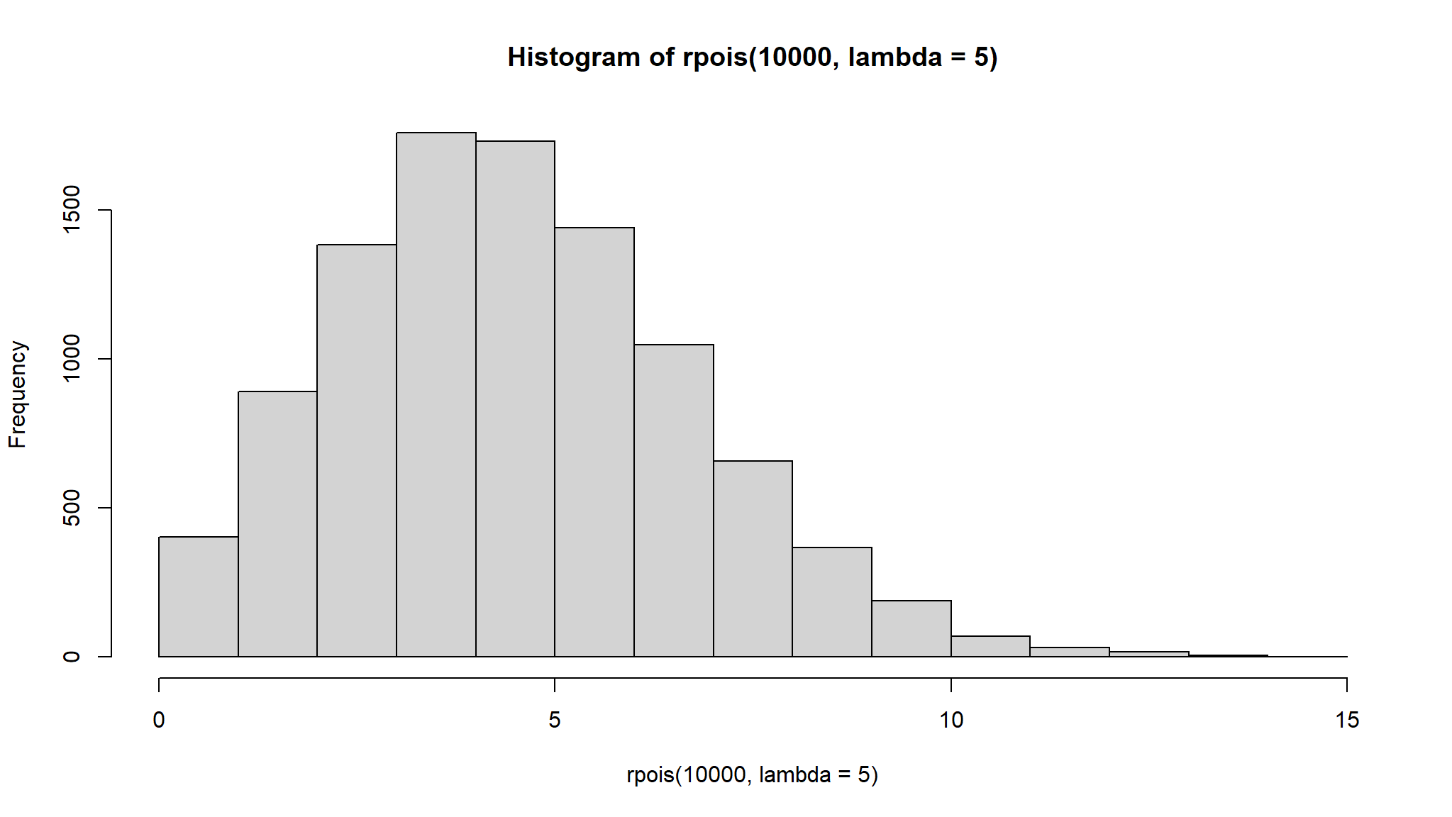
\(Pois(\lambda)\)
Density
\[ f(x) = \frac{e^{-k}k^x}{x!} \]
,k> 0, x =0,1,…
CDF
Use table
MGF
\[ m_X(t)=e^{k(e^t-1)} \]
Mean
\[ \mu = E(X) = k \]
Variance
\[ \sigma^2 = Var(X) = k \]
Density
\[ f(x)=pq^{x-1} \]
CDF
\[
F(x) = 1- q^x
\]
# hist of Geometric distribution with probability of success = 0.5
hist(rgeom(n = 10000, prob = 0.5))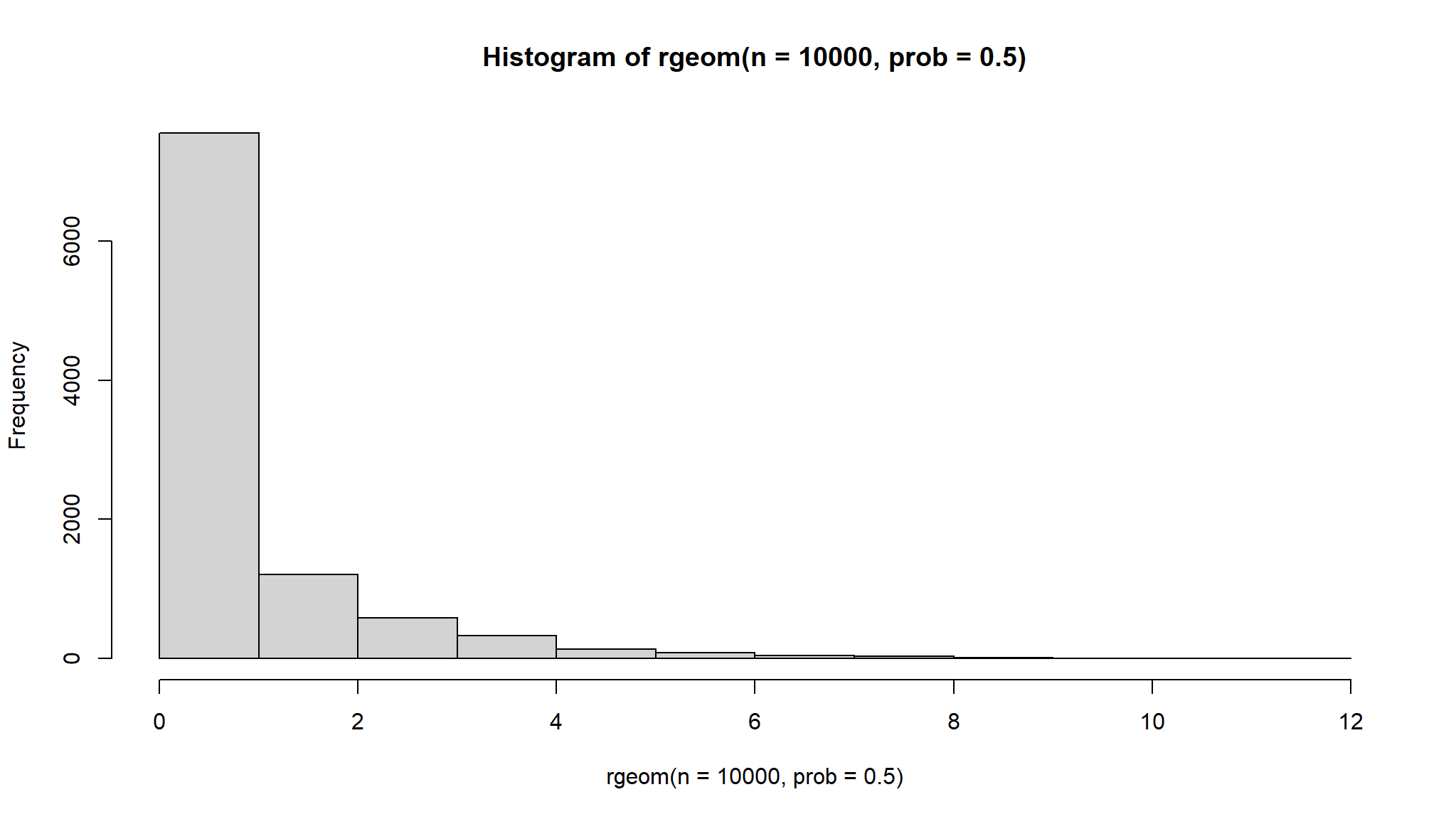
MGF
\[ m_X(t) = \frac{pe^t}{1-qe^t} \]
for \(t < -ln(q)\)
Mean
\[ \mu = \frac{1}{p} \]
Variance
\[ \sigma^2 = Var(X) = \frac{q}{p^2} \]
Density
\[ f(x)=\frac{{{r}\choose{x}}{{N-r}\choose{n-x}}}{{{N}\choose{n}}} \]
where \(max[0,n-(N-r)] \le x \le min(n,r)\)
# hist of hypergeometric distribution with the number of white balls = 50, and the number of black balls = 20, and number of balls drawn = 30.
hist(rhyper(nn = 10000 , m=50, n=20, k=30))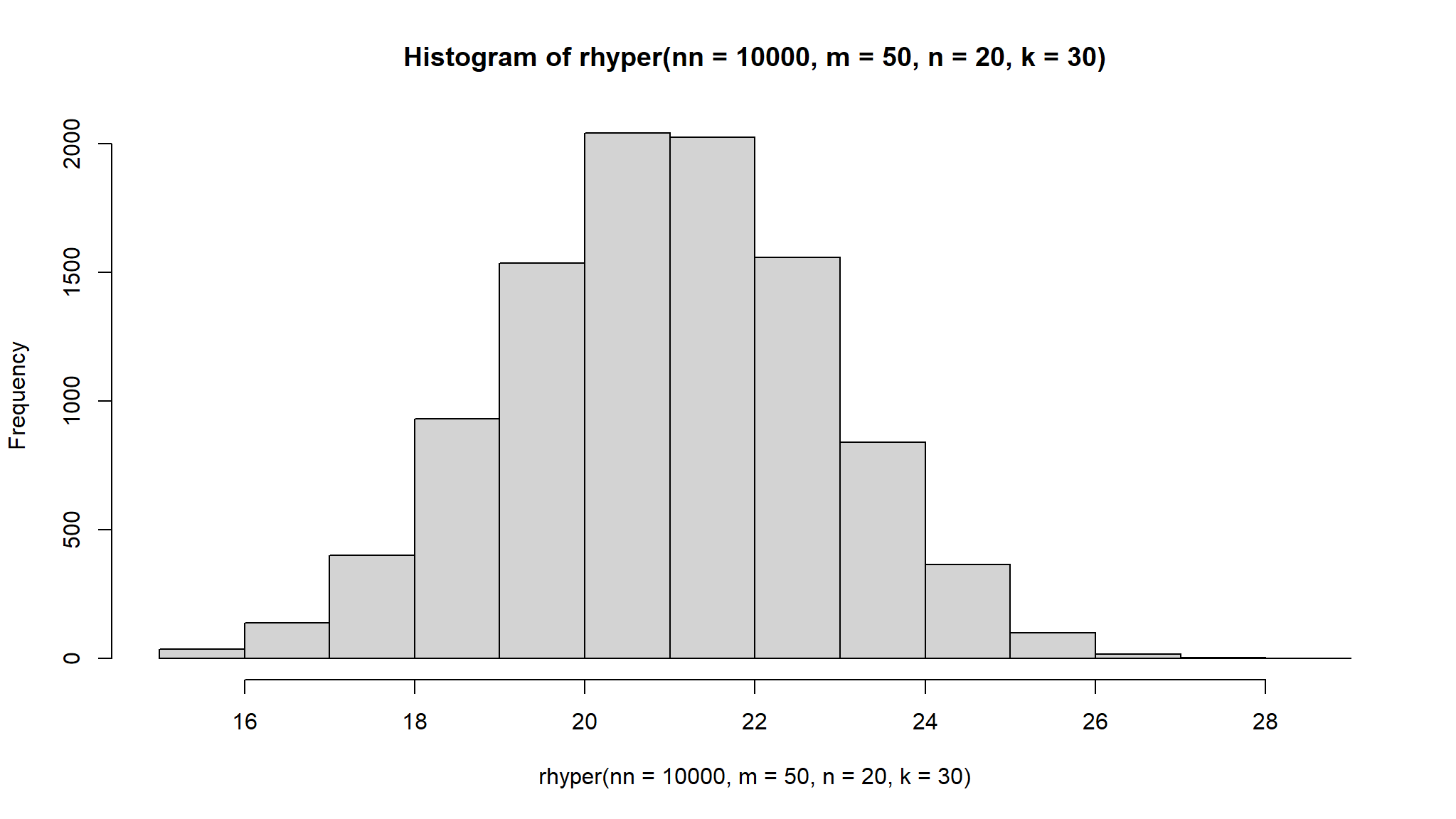
Mean
\[ \mu = E(x)= \frac{nr}{N} \]
Variance
\[ \sigma^2 = var(X) = n (\frac{r}{N})(\frac{N-r}{N})(\frac{N-n}{N-1}) \]
Note For large N (if \(\frac{n}{N} \le 0.05\)), this distribution can be approximated using a Binomial distribution with \(p = \frac{r}{N}\)
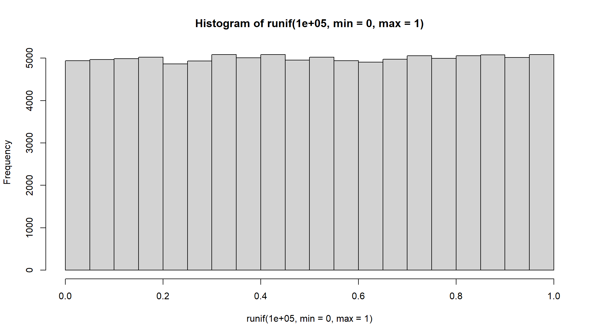
Density
\[ f(x)=\frac{1}{b-a} \]
for a < x < b
CDF
\[ \begin{cases} 0 & \text{if x <a } \\ \frac{x-a}{b-a} & \text{if $a \le x \le b$ }\\ 1 & \text{if x >b}\\ \end{cases} \]
MGF
\[ \begin{cases} \frac{e^{tb} - e^{ta}}{t(b-a)}&\text{ if $t \neq 0$}\\ 1&\text{if $ t \neq 0$}\\ \end{cases} \]
Mean
\[ \mu = E(X) = \frac{a +b}{2} \]
Variance
\[ \sigma^2 = Var(X) = \frac{(b-a)^2}{12} \]
\[ \Gamma(\alpha) = \int_0^{\infty} z^{\alpha-1}e^{-z}dz \]
where \(\alpha > 0\)
Properties of The Gamma function:
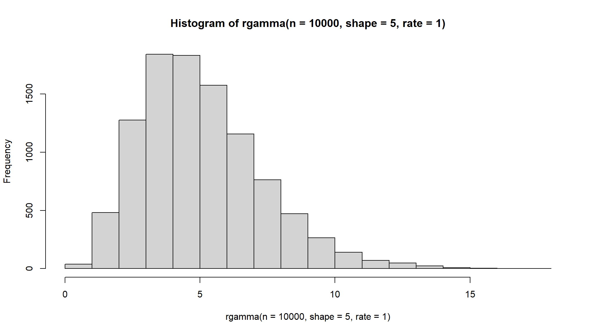
Density
\[ f(x) = \frac{1}{\Gamma(\alpha)\beta^{\alpha}}x^{\alpha-1}e^{-x/\beta} \]
CDF
\[ F(x,n,\beta) = 1 -\sum_{k=0}^{n-1} \frac{(\frac{x}{\beta})^k e^{-x/\beta}}{k!} \]
for x>0, and \(\alpha = n\) (a positive integer)
MGF
\[ m_X(t) = (1-\beta t)^{-\alpha} \]
where \(t < \frac{1}{\beta}\)
Mean
\[ \mu = E(X) = \alpha \beta \]
Variance
\[ \sigma^2 = Var(X) = \alpha \beta^2 \]
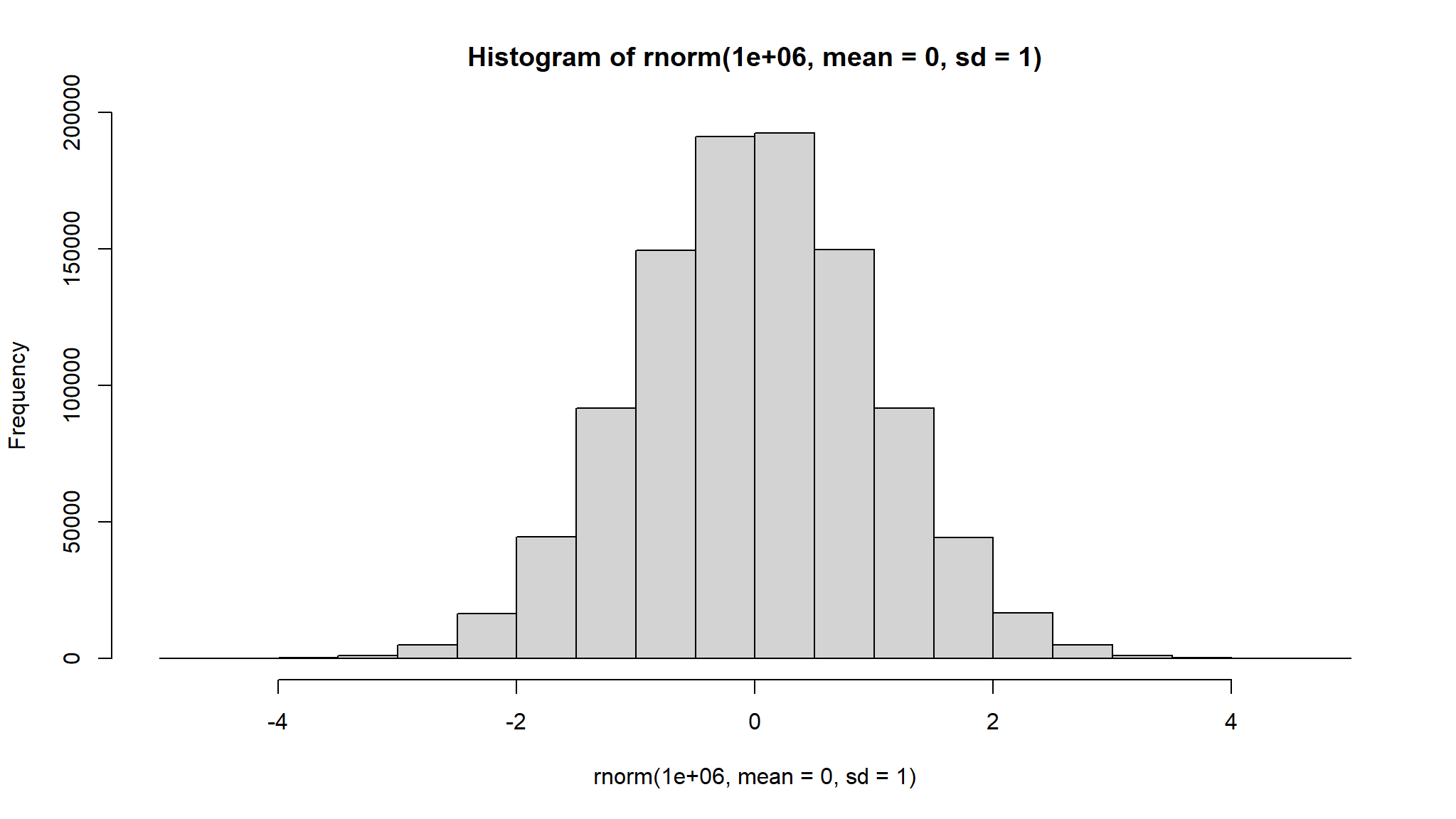
\(N(\mu,\sigma^2)\)
Density
\[ f(x) = \frac{1}{\sigma \sqrt{2\pi }}e^{-\frac{1}{2}(\frac{x-\mu}{\sigma})^2} \]
for \(-\infty < x, \mu< \infty, \sigma > 0\)
CDF
Use table
MGF
\[ m_X(t) = e^{\mu t + \frac{\sigma^2 t^2}{2}} \]
Mean
\[ \mu = E(X) \]
Variance
\[ \sigma^2 = Var(X) \]
Standard Normal Random Variable
Normal Approximation to the Binomial Distribution
Let X be binomial with parameters n and p. For large n (so that \((A)p \le .5\) and \(np > 5\) or (B) \(p>.5\) and \(nq>5\)), X is approximately normally distributed with mean \(\mu = np\) and standard deviation \(\sigma = \sqrt{npq}\)
When using the normal approximation, add or subtract 0.5 as needed for the continuity correction
| Discrete | Approximate Normal (corrected) |
|---|---|
| P(X = c) | P(c -0.5 < Y < c + 0.5) |
| P(X < c) | P(Y < c - 0.5) |
| P(X c) | P(Y < c + 0.5) |
| P(X > c) | P(Y > c + 0.5) |
| P(X c) | P(Y > c - 0.5) |
Normal Probability Rule
If X is normally distributed with parameters \(\mu\) and \(\sigma\), then
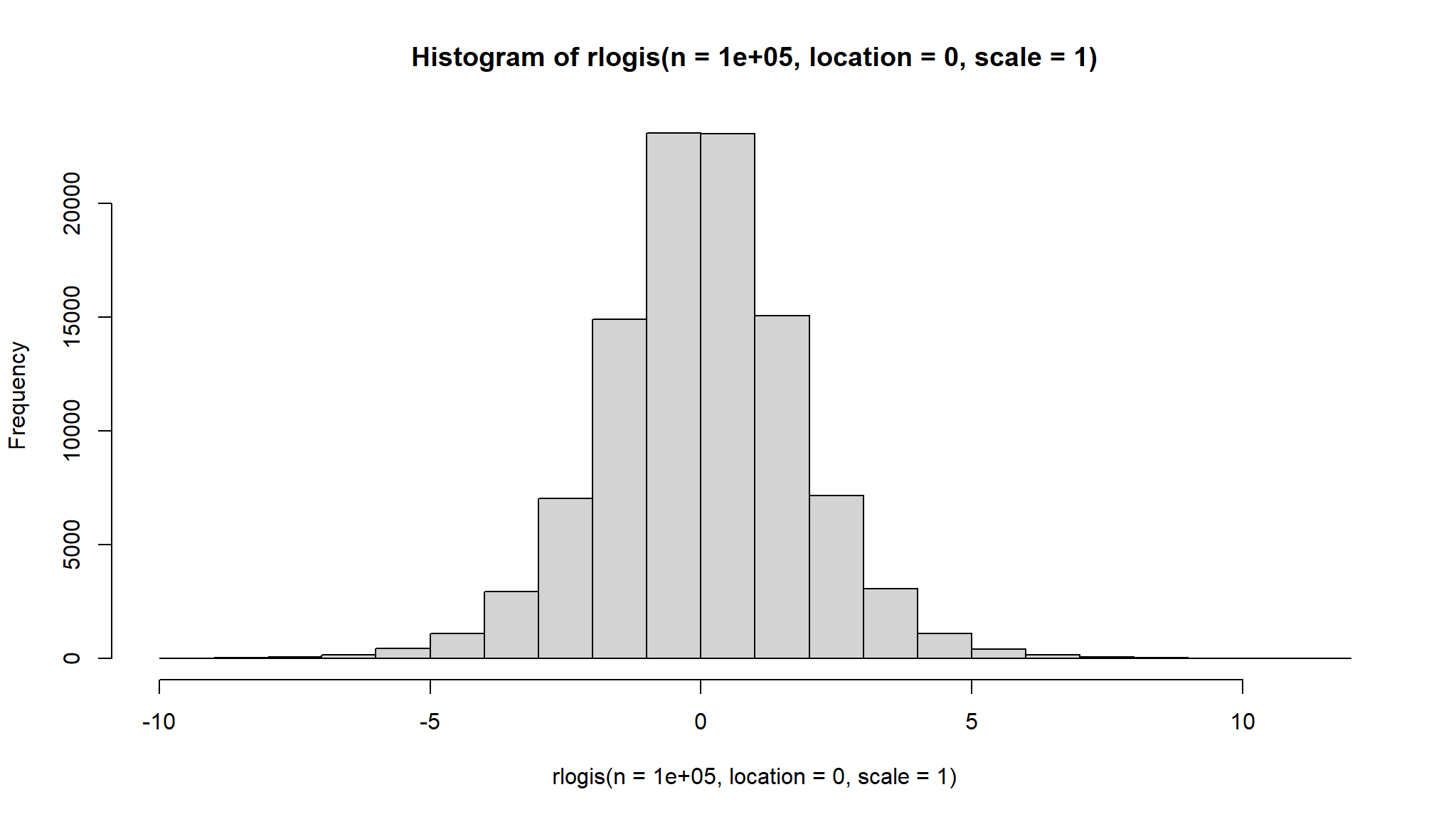
\(Logistic(\mu,s)\)
\[ f(x) = \frac{1}{2} e^{-|x-\theta|} \] where \(-\infty < x < \infty\) and \(-\infty < \theta < \infty\)
\[ \mu = \theta, \sigma^2 = 2 \] and
\[ m(t) = e^{t \theta} \frac{1}{1 - t^2} \] where \(-1 < t < 1\)
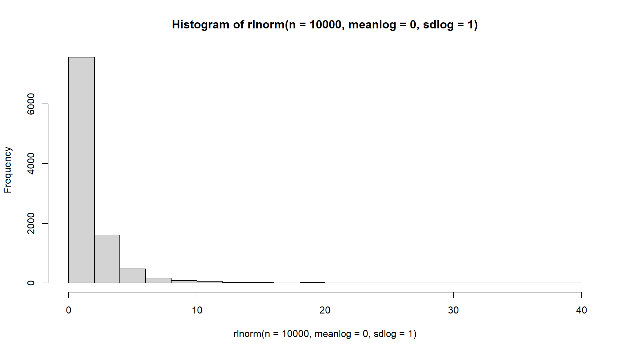
\(lognormal(\mu,\sigma^2)\)
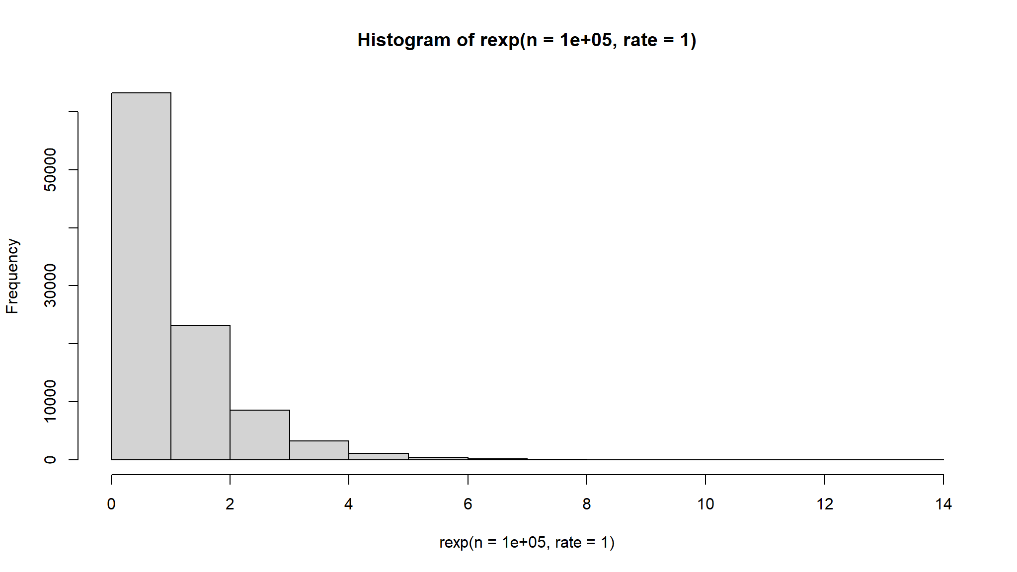
\(Exp(\lambda)\)
Density
\[ f(x) = \frac{1}{\beta} e^{-x/\beta} \]
for \(x,\beta > 0\)
CDF
\[\begin{equation} F(x) = \begin{cases} 0 & \text{ if $x \le 0$}\\ 1 - e^{-x/\beta} & \text{if $x > 0$}\\ \end{cases} \end{equation}\]
MGF
\[ m_X(t) = (1-\beta t)^{-1} \]
for \(t < 1/\beta\)
Mean
\[ \mu = E(X) = \beta \]
Variance
\[ \sigma^2 = Var(X) =\beta^2 \]
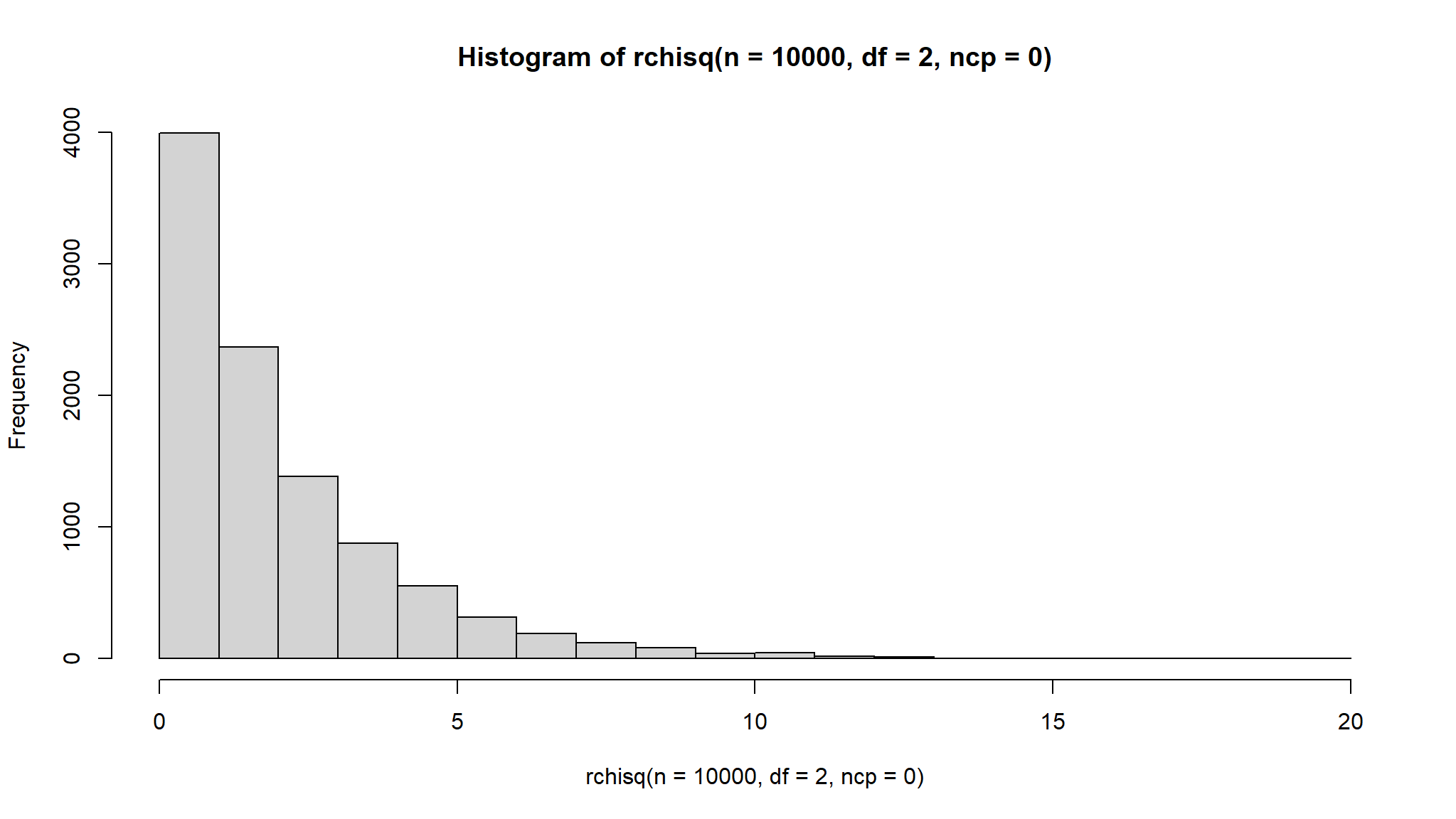
\(\chi^2=\chi^2(k)\)
Density Use density for Gamma Distribution with \(\beta = 2\) and \(\alpha = \gamma/2\)
CDF Use table
MGF
\[ m_X(t) = (1-2t)^{-\gamma/2} \]
Mean
\[ \mu = E(X) = \gamma \]
Variance
\[ \sigma^2 = Var(X) = 2\gamma \]
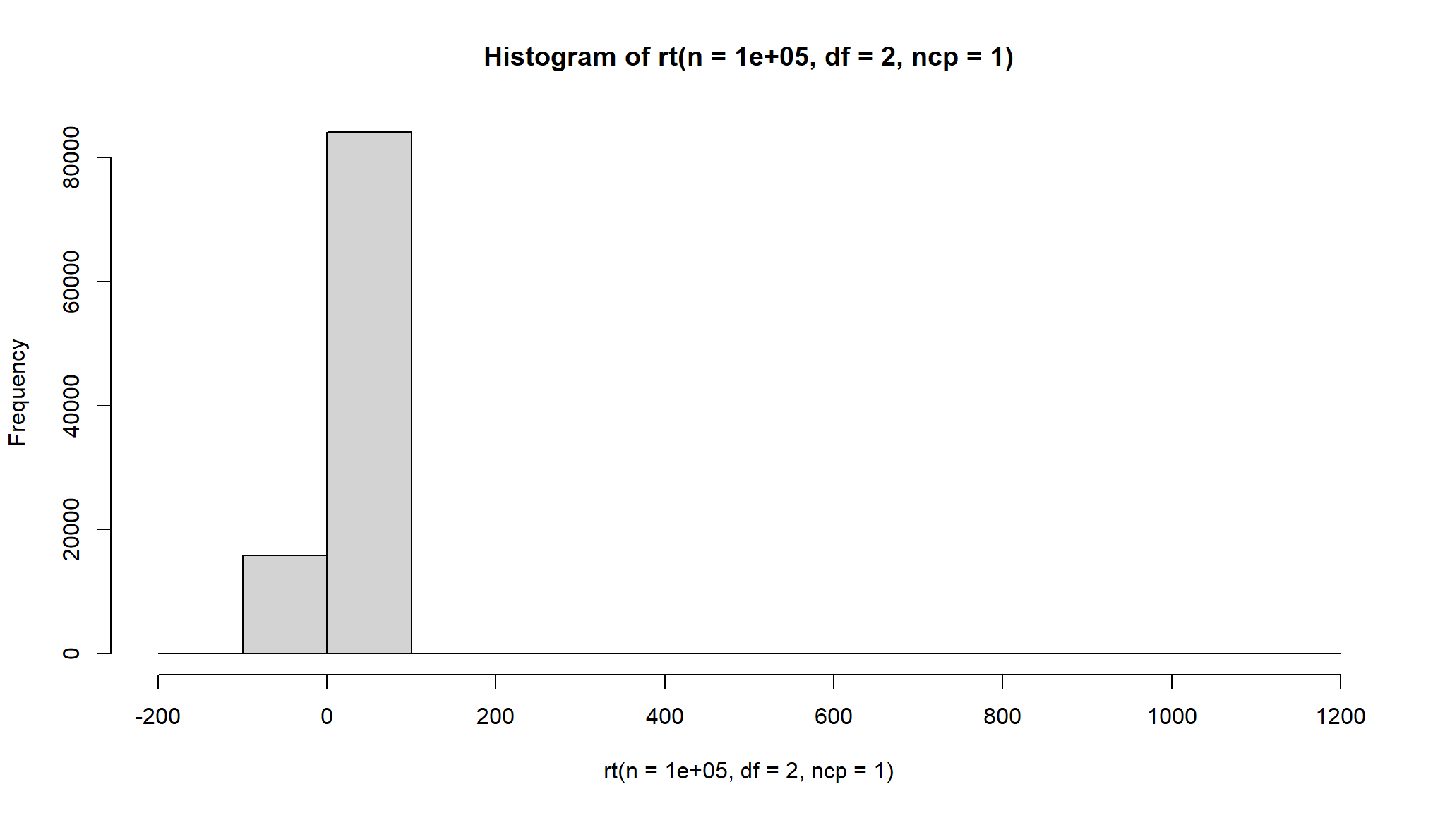
\(T(v)\)
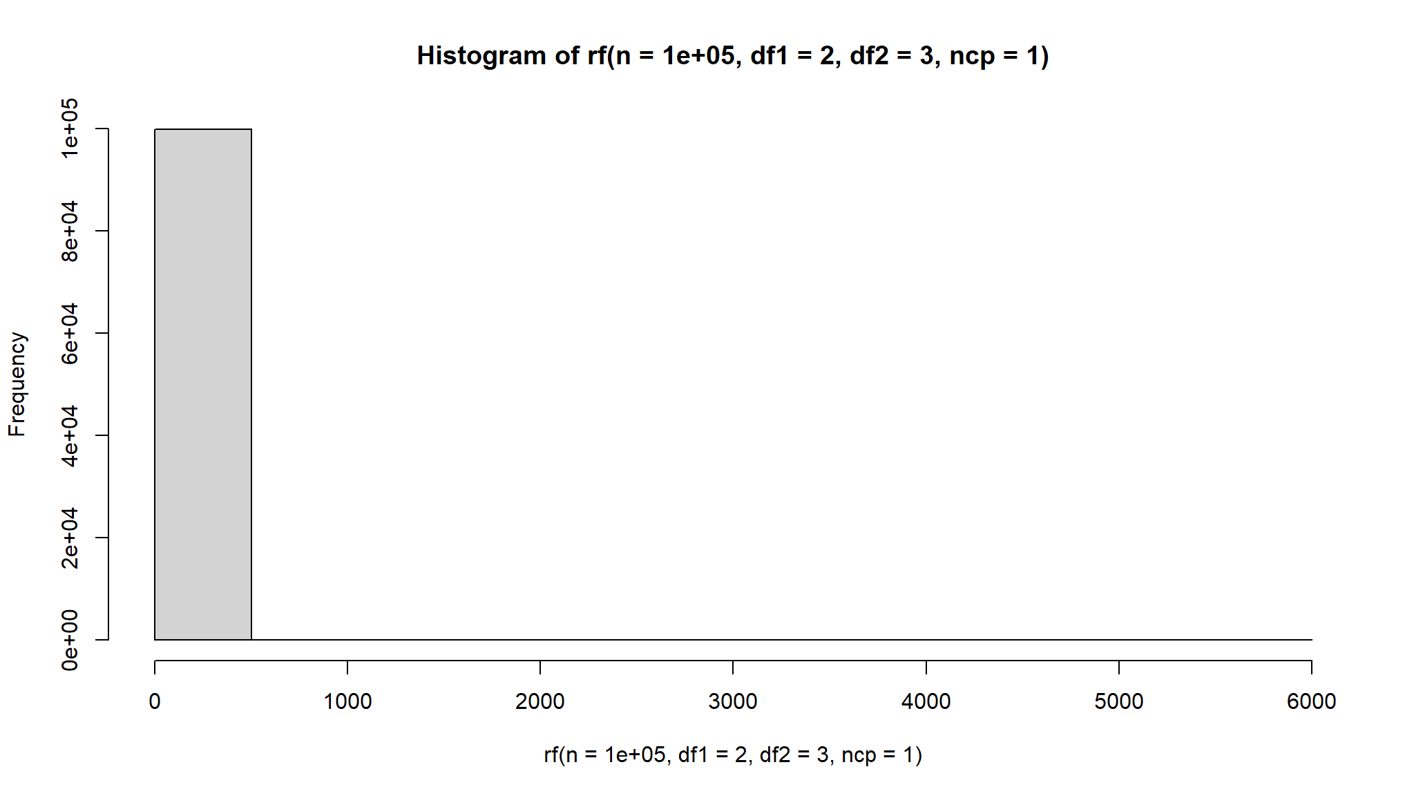
\(F(d_1,d_2)\)
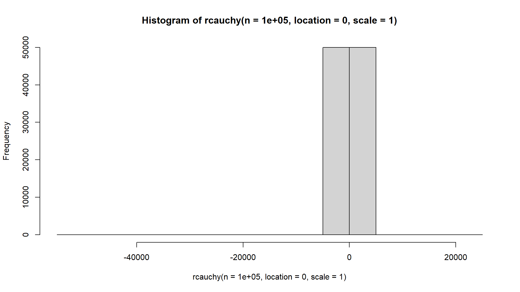
Central Limit Theorem and [Weak Law] do not apply to Cauchy because it does not have finite mean and finite variance
Let y be a p-dimensional multivariate normal (MVN) rv with mean \(\mu\) and variance \(\Sigma\). Then, the density of y is
\[ f(\mathbf{y}) = \frac{1}{(2\pi)^{p/2}|\mathbf{\Sigma}|^{1/2}}exp(-\frac{1}{2}\mathbf{(y-\mu)'\Sigma^{-1}(y-\mu)}) \]
We have \(\mathbf{y} \sim N_p(\mathbf{\mu,\Sigma})\)
Properties:
Large Sample Properties
Suppose that \(y_1,...,y_n\) are a random sample from some population with mean \(\mu\) and variance-variance matrix \(\Sigma\)
\[ \mathbf{Y} \sim MVN(\mathbf{\mu,\Sigma}) \]
Then