Rows: 731
Columns: 15
$ ...1 <dbl> 1, 2, 3, 4, 5, 6, 7, 8, 9, 10, 11, 12, 13, 14, 15, 16, 17, …
$ instant <dbl> 1, 2, 3, 4, 5, 6, 7, 8, 9, 10, 11, 12, 13, 14, 15, 16, 17, …
$ dteday <chr> "1/1/2011", "1/2/2011", "1/3/2011", "1/4/2011", "1/5/2011",…
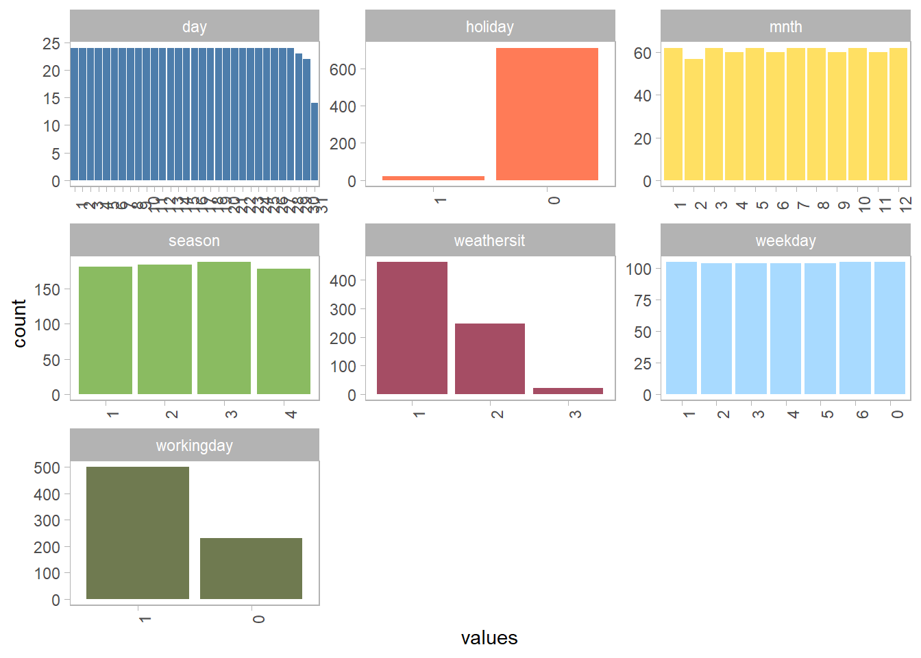
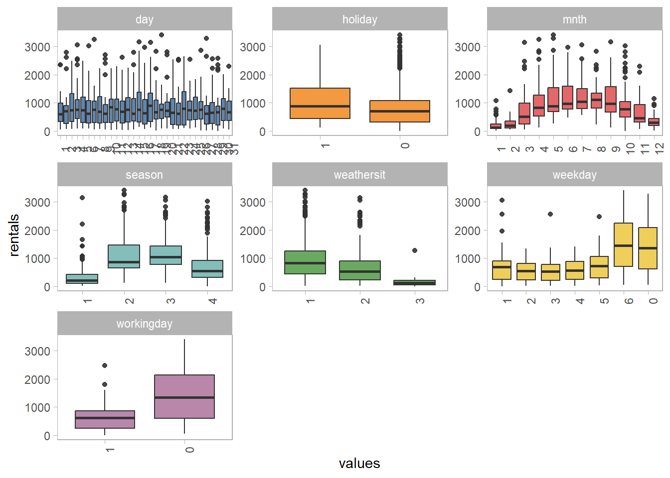
$ season <dbl> 1, 1, 1, 1, 1, 1, 1, 1, 1, 1, 1, 1, 1, 1, 1, 1, 1, 1, 1, 1,…
$ yr <dbl> 0, 0, 0, 0, 0, 0, 0, 0, 0, 0, 0, 0, 0, 0, 0, 0, 0, 0, 0, 0,…
$ mnth <dbl> 1, 1, 1, 1, 1, 1, 1, 1, 1, 1, 1, 1, 1, 1, 1, 1, 1, 1, 1, 1,…
$ holiday <dbl> 0, 0, 0, 0, 0, 0, 0, 0, 0, 0, 0, 0, 0, 0, 0, 0, 1, 0, 0, 0,…
$ weekday <dbl> 6, 0, 1, 2, 3, 4, 5, 6, 0, 1, 2, 3, 4, 5, 6, 0, 1, 2, 3, 4,…
$ workingday <dbl> 0, 0, 1, 1, 1, 1, 1, 0, 0, 1, 1, 1, 1, 1, 0, 0, 0, 1, 1, 1,…
$ weathersit <dbl> 2, 2, 1, 1, 1, 1, 2, 2, 1, 1, 2, 1, 1, 1, 2, 1, 2, 2, 2, 2,…
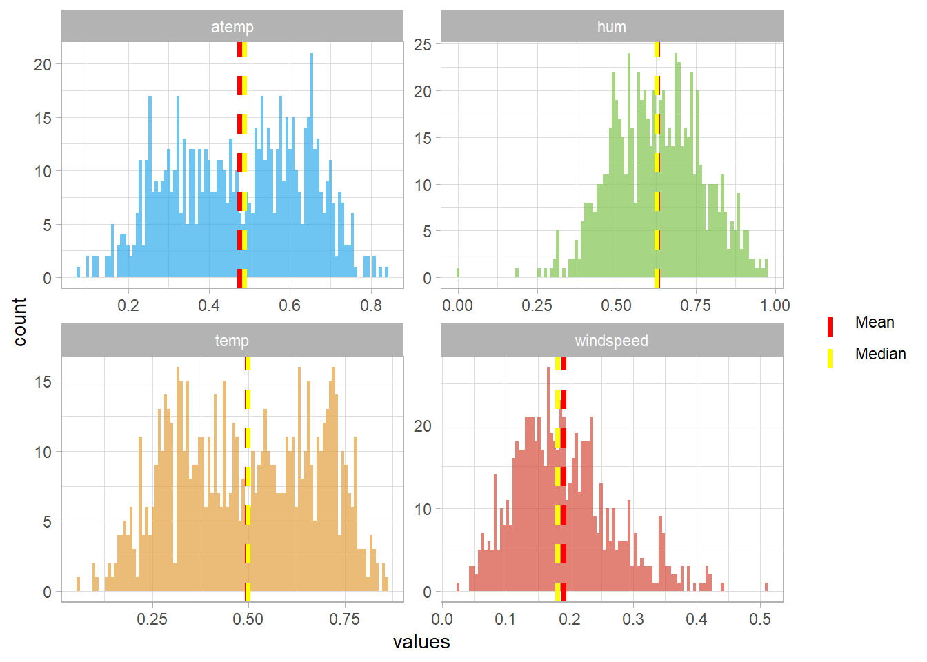
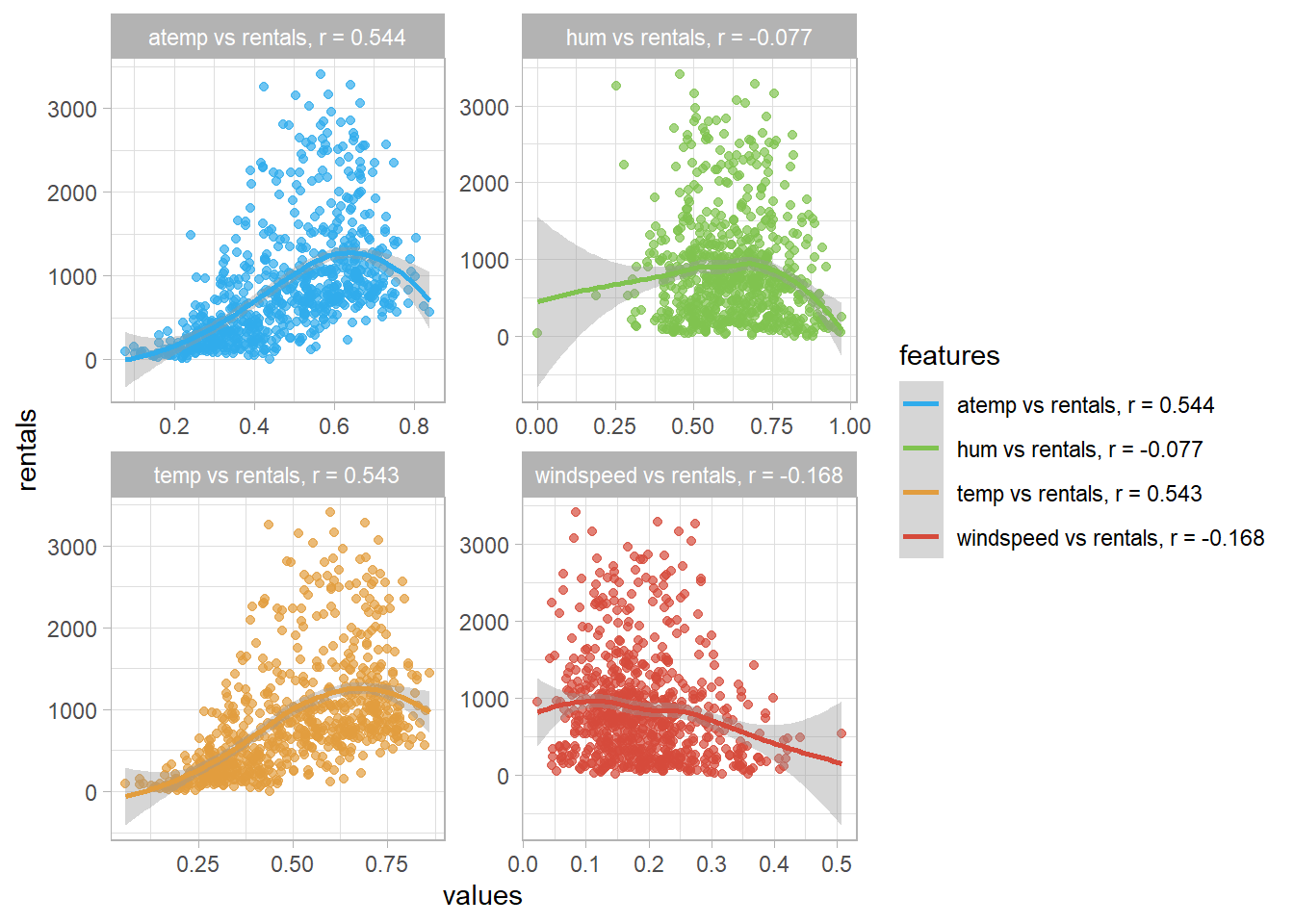
$ temp <dbl> 0.3441670, 0.3634780, 0.1963640, 0.2000000, 0.2269570, 0.20…
$ atemp <dbl> 0.3636250, 0.3537390, 0.1894050, 0.2121220, 0.2292700, 0.23…
$ hum <dbl> 0.805833, 0.696087, 0.437273, 0.590435, 0.436957, 0.518261,…
$ windspeed <dbl> 0.1604460, 0.2485390, 0.2483090, 0.1602960, 0.1869000, 0.08…
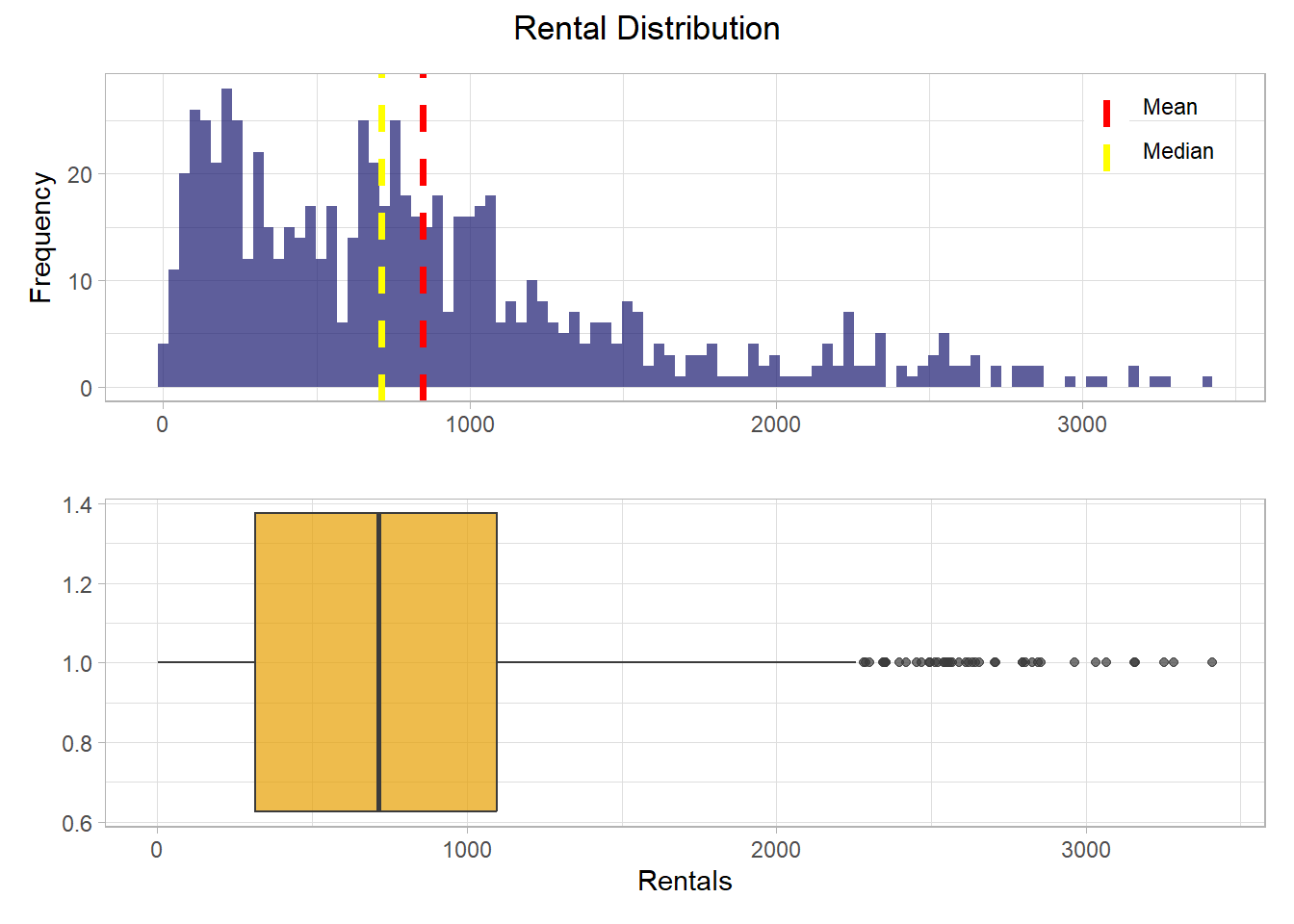
$ rentals <dbl> 331, 131, 120, 108, 82, 88, 148, 68, 54, 41, 43, 25, 38, 54…
comments