Comparing and Ensembling Machine Learning Models

Predicting Airbnb prices

Introduction

Machine Learning

Stats

Random Forest

XGBoost

SVM

KNN

Building different Models and Intercomparing, and then Combining into an Ensemble

Author

Bongani Ncube

Published

3 October 2025

Introduction

I once carried out a study using this data on B Ncube Analysis

my_data<-readr::read_csv("airbnb_data.csv")
DT::datatable(my_data,filter="top")

Data Cleaning

out_new<-my_data |> 
  mutate(neighbourhood_location=
           case_when(str_detect(neighbourhood_full,"Staten Island")~"Staten Island",
                     str_detect(neighbourhood_full,"Queens")~"Queens",
                     str_detect(neighbourhood_full,"Manhattan")~"Manhattan",
                     str_detect(neighbourhood_full,"Brooklyn")~"Brooklyn",
                     str_detect(neighbourhood_full,"Bronx")~"Bronx"))

Count of neighborhoods

out_new |> 
  janitor::tabyl(neighbourhood_location) |> 
  as_tibble() |> 
  arrange(desc(n)) |> 
  ggplot(aes(x=fct_reorder(neighbourhood_location, n), n)) +
  geom_col() + 
  scale_fill_avatar()+
  theme_avatar()+
  labs(x="Neighborhood", 
       y="count", 
       title="") + 
  coord_flip() + 
  geom_text(aes(label=paste0(round(n), "x "), hjust=1), col="purple")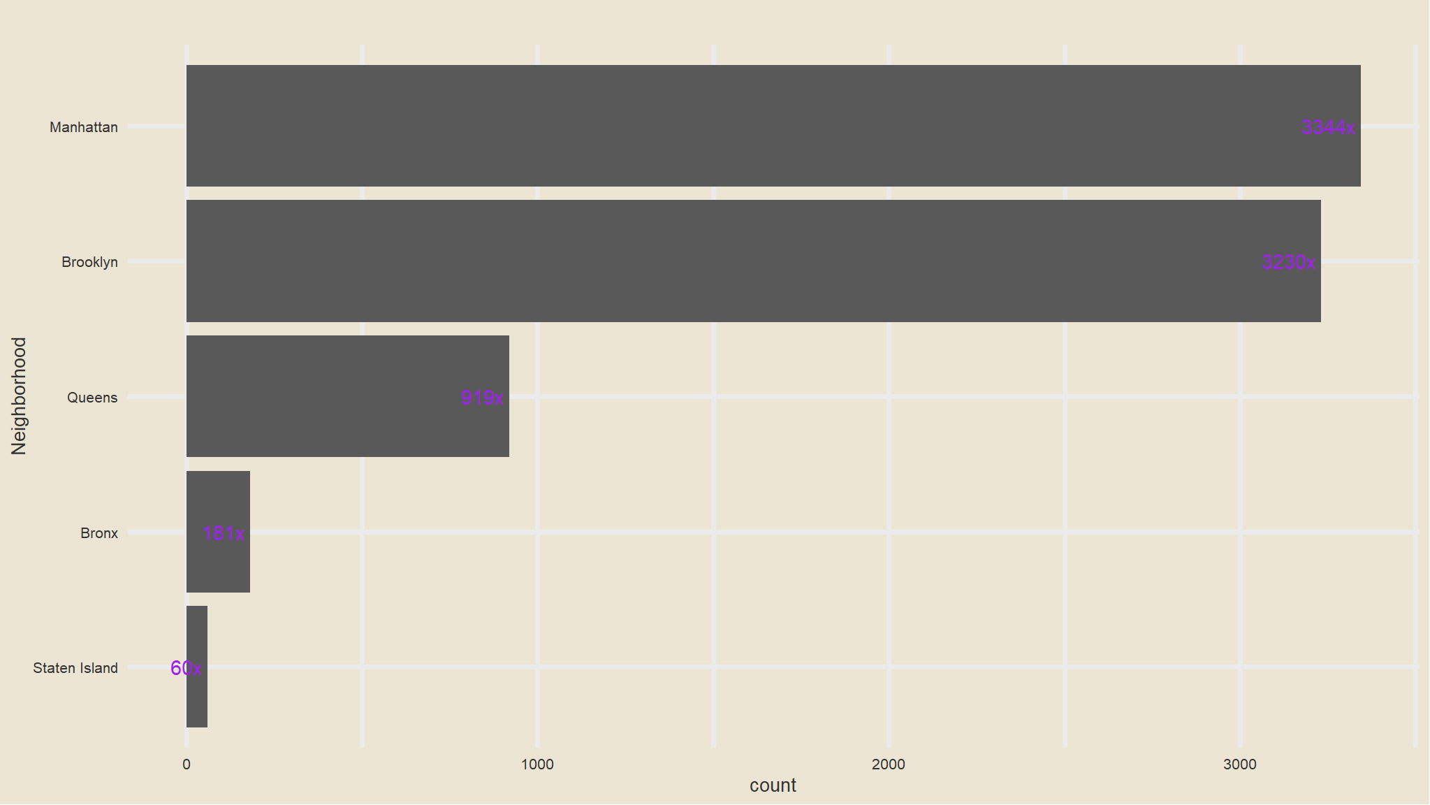

Note

Comments

that is now better , we seem to have managable categories now.
Manhattan has the greatest number of listings

Mean Price comparison in Each neighborhood

out_new |> 
  group_by(neighbourhood_location) |> 
  summarise(avg=mean(price)) |> 
  ggplot(aes(x=fct_reorder(neighbourhood_location, avg), avg)) +
  geom_col() + 
  scale_fill_avatar()+
  theme_avatar()+
  labs(x="Neighborhood", 
       y="Average", 
       title="") + 
  coord_flip() + 
  geom_text(aes(label=paste0(round(avg), "$"), hjust=1), col="purple")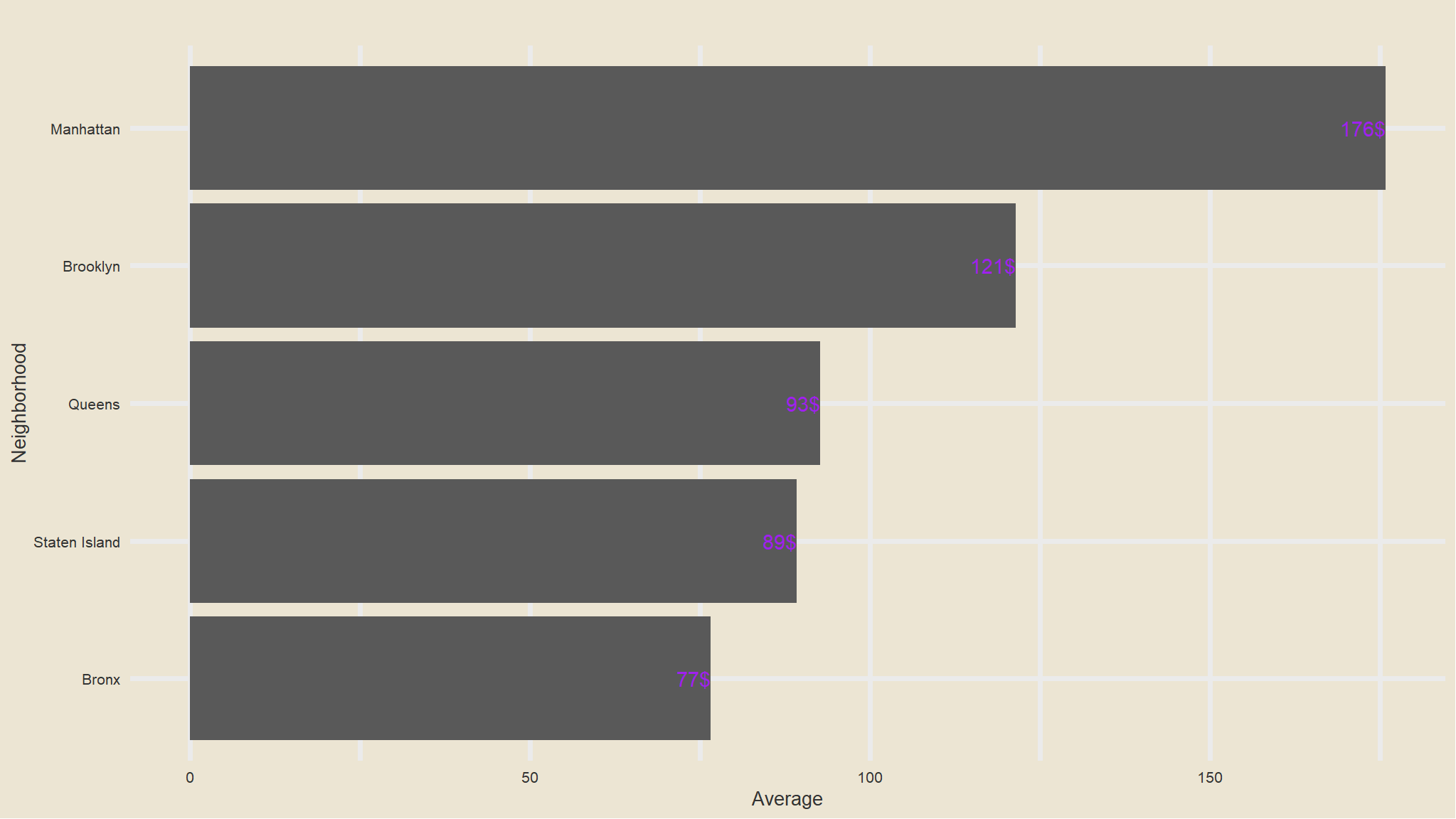

Note

Comments

average price listings is highest in Manhattan followed by Brooklyn this could be due to the fact that the most common type of listings is the entire apartment
Bronx Has the cheapest listings as compared to others

Mean Price comparison in Each room type

out_new |> 
  group_by(room_type) |> 
  summarise(avg=mean(price)) |> 
  ggplot(aes(x=fct_reorder(room_type, avg), avg)) +
  geom_col() + 
  scale_fill_avatar()+
  theme_avatar()+
  labs(x="Room Type", 
       y="Average", 
       title="") + 
  coord_flip() + 
  geom_text(aes(label=paste0(round(avg), "$"), hjust=1), col="purple")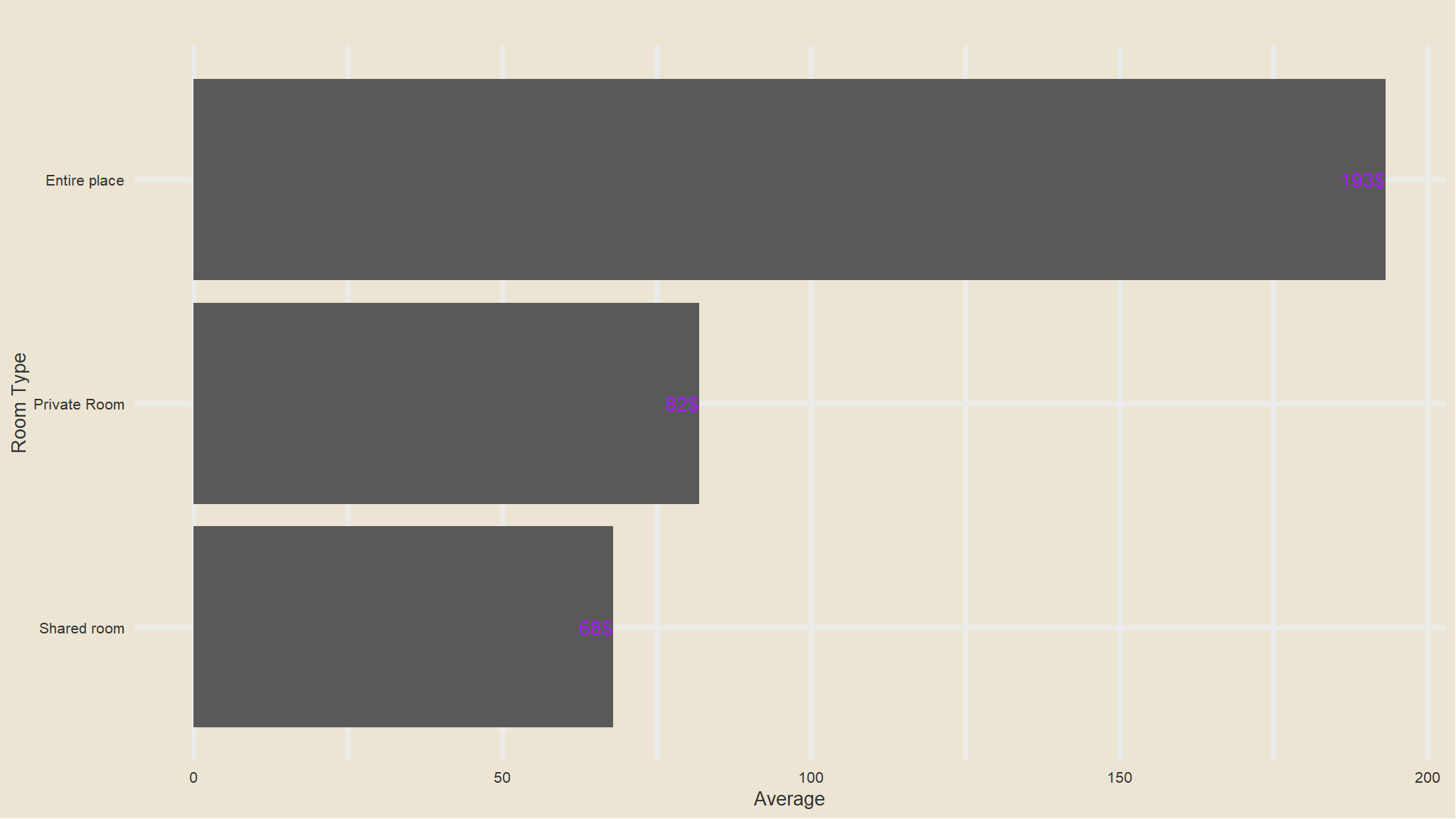

Note

Comments

Whole apartments have the largest prices compared to other rooms , this is really expected

Geospatial data

out_new 
#> # A tibble: 7,734 × 14
#>    listing_id description host_id neighbourhood_full coordinates room_type price
#>         <dbl> <chr>         <dbl> <chr>              <chr>       <chr>     <dbl>
#>  1   13740704 Cozy,budge…  2.06e7 Brooklyn, Flatlan… (40.63222,… Private …    45
#>  2   22005115 Two floor …  8.27e7 Manhattan, Upper … (40.78761,… Entire p…   135
#>  3    6425850 Spacious, …  3.27e7 Manhattan, Upper … (40.79169,… Entire p…    86
#>  4   22986519 Bedroom on…  1.54e8 Manhattan, Lower … (40.71884,… Private …   160
#>  5     271954 Beautiful …  1.42e6 Manhattan, Greenw… (40.73388,… Entire p…   150
#>  6   14218742 Luxury/3be…  7.88e7 Brooklyn, Sheepsh… (40.58531,… Entire p…   224
#>  7   15125599 Beautiful …  3.19e6 Manhattan, Theate… (40.761, -… Entire p…   169
#>  8   24553891 Enjoy all …  6.86e7 Manhattan, Harlem  (40.80667,… Entire p…    75
#>  9   26386759 Cozy and e…  8.69e7 Brooklyn, Bushwick (40.70103,… Private …    50
#> 10   34446664 Home away …  2.60e8 Queens, Laurelton  (40.6688, … Entire p…   254
#> # ℹ 7,724 more rows
#> # ℹ 7 more variables: number_of_reviews <dbl>, reviews_per_month <dbl>,
#> #   availability_365 <dbl>, rating <dbl>, number_of_stays <dbl>,
#> #   listing_added <date>, neighbourhood_location <chr>

out_new |> 
  separate(coordinates,into=c("lAT","LONG"),sep=",") |> 
  relocate(lAT,LONG)
#> # A tibble: 7,734 × 15
#>    lAT   LONG  listing_id description host_id neighbourhood_full room_type price
#>    <chr> <chr>      <dbl> <chr>         <dbl> <chr>              <chr>     <dbl>
#>  1 (40.… " -7…   13740704 Cozy,budge…  2.06e7 Brooklyn, Flatlan… Private …    45
#>  2 (40.… " -7…   22005115 Two floor …  8.27e7 Manhattan, Upper … Entire p…   135
#>  3 (40.… " -7…    6425850 Spacious, …  3.27e7 Manhattan, Upper … Entire p…    86
#>  4 (40.… " -7…   22986519 Bedroom on…  1.54e8 Manhattan, Lower … Private …   160
#>  5 (40.… " -7…     271954 Beautiful …  1.42e6 Manhattan, Greenw… Entire p…   150
#>  6 (40.… " -7…   14218742 Luxury/3be…  7.88e7 Brooklyn, Sheepsh… Entire p…   224
#>  7 (40.… " -7…   15125599 Beautiful …  3.19e6 Manhattan, Theate… Entire p…   169
#>  8 (40.… " -7…   24553891 Enjoy all …  6.86e7 Manhattan, Harlem  Entire p…    75
#>  9 (40.… " -7…   26386759 Cozy and e…  8.69e7 Brooklyn, Bushwick Private …    50
#> 10 (40.… " -7…   34446664 Home away …  2.60e8 Queens, Laurelton  Entire p…   254
#> # ℹ 7,724 more rows
#> # ℹ 7 more variables: number_of_reviews <dbl>, reviews_per_month <dbl>,
#> #   availability_365 <dbl>, rating <dbl>, number_of_stays <dbl>,
#> #   listing_added <date>, neighbourhood_location <chr>

interesting , note that i am doing this the easisest and most understandable way

next up i need to remove the brackets and save the whole thing into an object

out_new<-out_new |> 
  separate(coordinates,into=c("lAT","LONG"),sep=",") |> 
  relocate(lAT,LONG) |> 
  mutate(lAT=readr::parse_number(lAT),
         LONG=readr::parse_number(LONG))
out_new
#> # A tibble: 7,734 × 15
#>      lAT  LONG listing_id description host_id neighbourhood_full room_type price
#>    <dbl> <dbl>      <dbl> <chr>         <dbl> <chr>              <chr>     <dbl>
#>  1  40.6 -73.9   13740704 Cozy,budge…  2.06e7 Brooklyn, Flatlan… Private …    45
#>  2  40.8 -74.0   22005115 Two floor …  8.27e7 Manhattan, Upper … Entire p…   135
#>  3  40.8 -74.0    6425850 Spacious, …  3.27e7 Manhattan, Upper … Entire p…    86
#>  4  40.7 -74.0   22986519 Bedroom on…  1.54e8 Manhattan, Lower … Private …   160
#>  5  40.7 -74.0     271954 Beautiful …  1.42e6 Manhattan, Greenw… Entire p…   150
#>  6  40.6 -73.9   14218742 Luxury/3be…  7.88e7 Brooklyn, Sheepsh… Entire p…   224
#>  7  40.8 -74.0   15125599 Beautiful …  3.19e6 Manhattan, Theate… Entire p…   169
#>  8  40.8 -74.0   24553891 Enjoy all …  6.86e7 Manhattan, Harlem  Entire p…    75
#>  9  40.7 -73.9   26386759 Cozy and e…  8.69e7 Brooklyn, Bushwick Private …    50
#> 10  40.7 -73.7   34446664 Home away …  2.60e8 Queens, Laurelton  Entire p…   254
#> # ℹ 7,724 more rows
#> # ℹ 7 more variables: number_of_reviews <dbl>, reviews_per_month <dbl>,
#> #   availability_365 <dbl>, rating <dbl>, number_of_stays <dbl>,
#> #   listing_added <date>, neighbourhood_location <chr>

cases<-complete.cases(out_new)
out_new_data<-out_new[cases,]
out_new_data<-out_new_data |> 
  dplyr::filter(price<2000) |> 
  dplyr::select(-host_id,-listing_id,-neighbourhood_full,-listing_added,-description,-number_of_reviews,-lAT,-LONG) |> 
  mutate_if(is.character,as.factor)

Building a Regression Model

# Load the Tidymodels packages
library(tidymodels)

# Split 70% of the data for training and the rest for tesing
set.seed(2056)
abnb_split <- out_new_data %>% 
  initial_split(prop = 0.7,
  # splitting data evenly on the holiday variable
                strata = price)

# Extract the data in each split
abnb_train <- training(abnb_split)
abnb_test <- testing(abnb_split)

glue::glue(
  'Training Set: {nrow(abnb_train)} rows
  Test Set: {nrow(abnb_test)} rows')
#> Training Set: 5403 rows
#> Test Set: 2318 rows

Data Splitting


folds<-vfold_cv(abnb_train,v=5)

Create Recipe

First we want to create a recipe that takes all columns (apart from id) to predict the average ranking. We also square root transform max players as some have huge max players.


recipe<-recipe(price~.,data=abnb_train) |> 
  step_dummy(all_nominal_predictors())

Create Model Specification

This is the first step where we choose the models we will compare. Lets do a glm, random forest, XGBoost, SVM and KNN.


glm_spec<-linear_reg(
  penalty = tune(), 
  mixture = tune()) %>% 
  set_mode("regression")%>%
  set_engine("glmnet")

rf_spec<- rand_forest(
  mtry = tune(),
  trees = tune(),
  min_n = tune()
) %>%
  set_mode("regression") %>%
  set_engine("ranger")

xgboost_spec<-boost_tree(
    trees = tune(),
    mtry = tune(),
    min_n = tune(),
    learn_rate = tune()
  ) %>%
  set_mode("regression")%>%
  set_engine("xgboost") 

# install.packages("kknn")
# install.packages("kernlab")

svm_spec<-  svm_rbf(
  cost = tune(), 
  rbf_sigma = tune()
  ) %>%
  set_mode("regression") %>%
  set_engine("kernlab")

knn_spec<-nearest_neighbor(neighbors = tune())%>%
  set_mode("regression") %>% 
  set_engine("kknn")

Model Hyper Parameter Tuning

So we could train each of these models as separate workflows then assess hyper parameter tuning as follows.


glm_wf<-workflow() %>%
  add_recipe(recipe) %>%
  add_model(glm_spec)


tune_res_glm <- tune_grid(
  glm_wf,
  resamples = folds,
  grid = 5
)

tune_res_glm %>%
  collect_metrics() %>%
  filter(.metric == "rmse") %>%
  dplyr::select(mean, penalty, mixture) %>%
  pivot_longer(penalty:mixture,
    values_to = "value",
    names_to = "parameter"
  ) %>%
  ggplot(aes(value, mean, color = parameter)) +
  geom_point(show.legend = FALSE) +
  facet_wrap(~parameter, scales = "free_x") +
  labs(x = NULL, y = "RMSE")+
  theme_classic()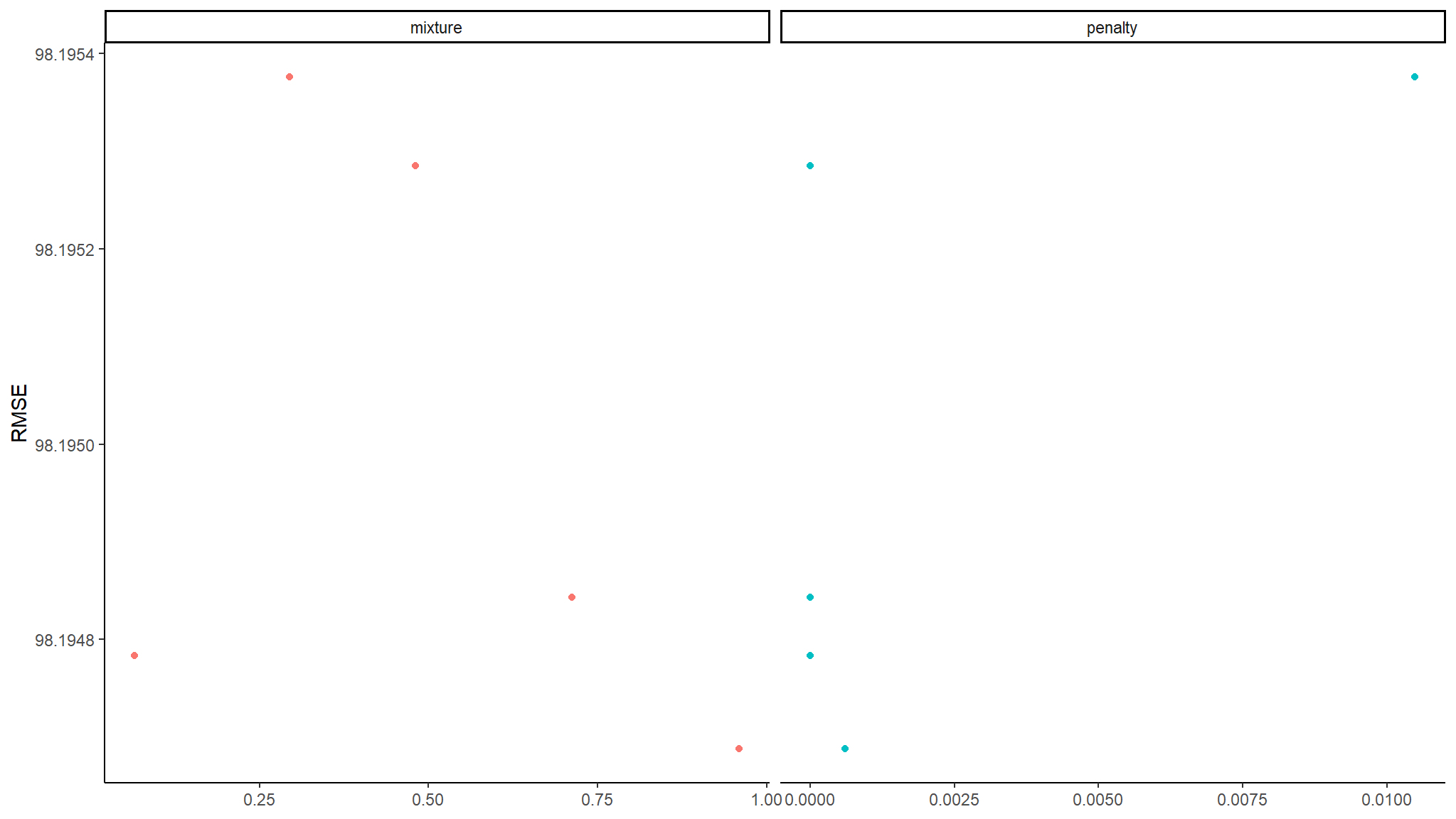

But we will be comparing lots of specs of models so lets make a workflowset and then do the same but with lots of trained models. This will take a long time, so i set the grid to be just 5, really it should be set to around 10, or you can use other methods other than grid search. We will also add (using option_add()) a control to the grid being used and the metric to be assessed (this will be necessary when we want to ensemble the models).

metric <- metric_set(rmse)

set.seed(234)

doParallel::registerDoParallel()

all_wf<-workflow_set(
  list(recipe),
  list(glm_spec,
       rf_spec,
       xgboost_spec,
       svm_spec,
       knn_spec)) %>%
  option_add(
    control = control_stack_grid(),
    metrics = metric
  )

all_res<- all_wf %>% 
  workflow_map(
    resamples=folds,
    grid=10
  )

Once that finishes running we can compare between all the tuned models.


autoplot(
   all_res,
   rank_metric = "rmse",  # <- how to order models
   metric = "rmse",       # <- which metric to visualize
   select_best = TRUE     # <- one point per workflow
) +geom_text(aes(y = mean - 0.075, label = wflow_id), angle = 80, hjust = 1)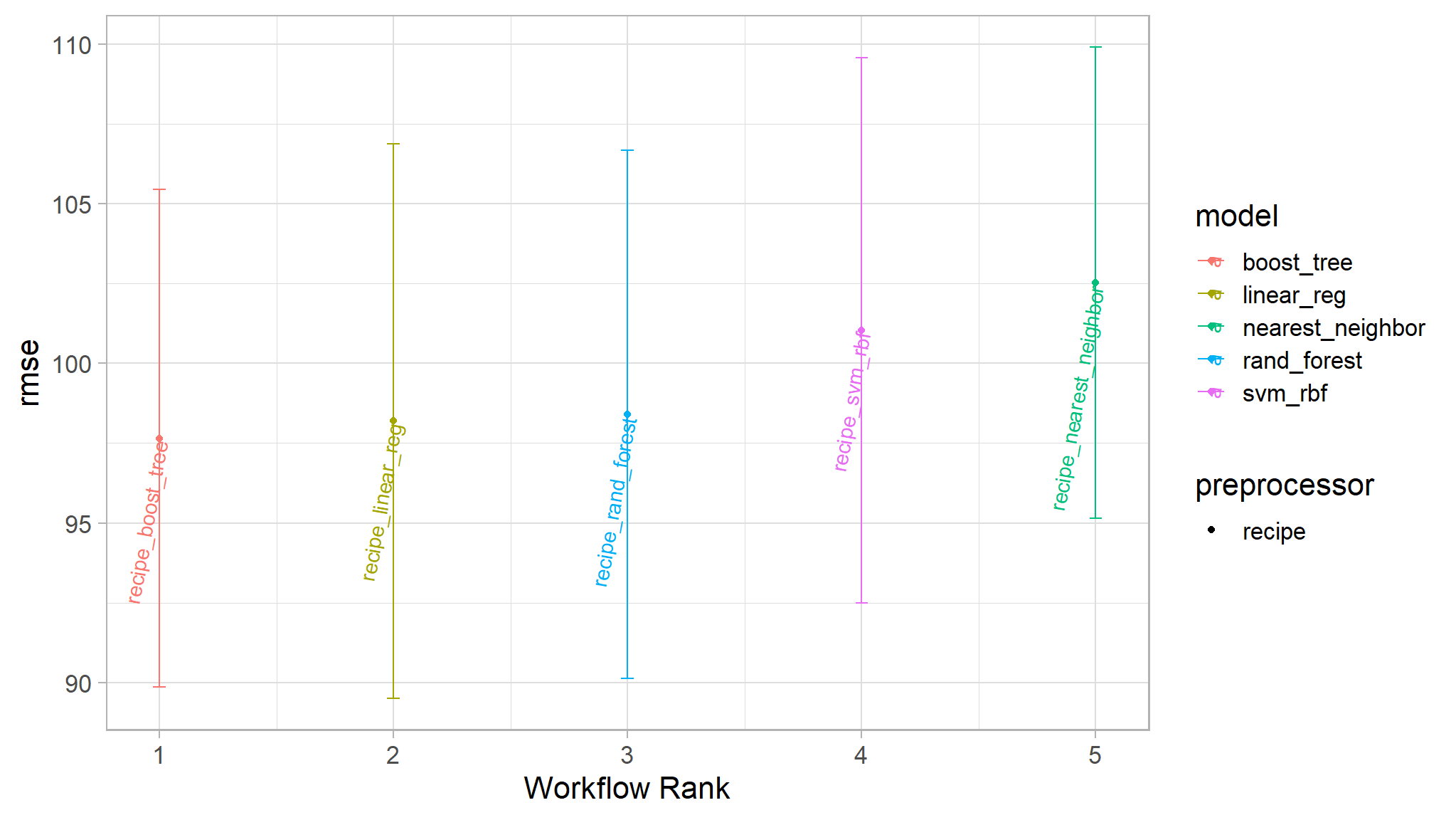

Select Best Model

Lets select a good model, then see how well it performs on predicting the test data. All models performed fairly well but lets select the recipe_boost_tree model. The best_results object provides us the ‘best’ hyper parameter values for this model framework (the best hyper parameters for the boosted tree models looked at). This is based on a very small amount of tests here, in reality we should use many more combinations of hyper parameters to test the best ones.


best_results <- all_res %>% 
   extract_workflow_set_result("recipe_boost_tree") %>% 
   select_best(metric = "rmse")

best_results
#> # A tibble: 1 × 5
#>    mtry trees min_n learn_rate .config              
#>   <int> <int> <int>      <dbl> <chr>                
#> 1     2  1333    39    0.00850 Preprocessor1_Model02

Assess Ability of ‘Best’ Model

Now lets combine these hyperparrameter values with the workflow, finalise the model and then fit to the initial split of our data. Then we can collect the metrics when this model was applied to the test dataset.


boosting_test_results <- 
   all_res %>% 
   extract_workflow("recipe_boost_tree") %>% 
   finalize_workflow(best_results) %>% 
   last_fit(split =abnb_split)
  
collect_metrics(boosting_test_results)
#> # A tibble: 2 × 4
#>   .metric .estimator .estimate .config             
#>   <chr>   <chr>          <dbl> <chr>               
#> 1 rmse    standard     108.    Preprocessor1_Model1
#> 2 rsq     standard       0.257 Preprocessor1_Model1

We can also plot the predicted verses the true results.


boosting_test_results %>% 
   collect_predictions() %>% 
   ggplot(aes(x = price , y = .pred)) + 
   geom_abline(colour = "gray50", linetype = 2) + 
   geom_pointdensity() + 
   coord_obs_pred()+
  scale_color_viridis() + 
   labs(x = "Observed", y = "Predicted",colour="Density")+
   theme_classic()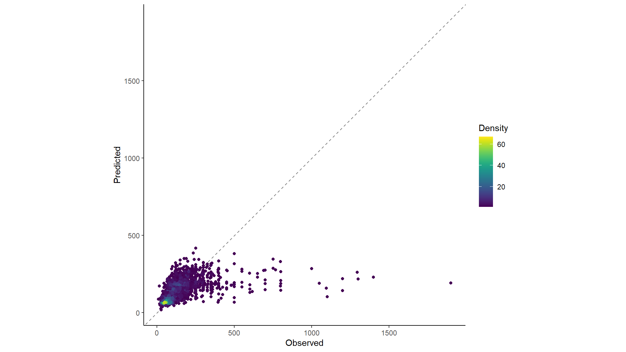

Ensemble All Models Together

After training all these different models and there could be a lot more, we may be losing predictive ability by only selecting the best one. It has been shown by many researchers that combining an ensemble of models will generally lead to better prediction ability. With the Stacks package in r we can easily stack or ensemble our models together.



 all_stacked<-stacks() %>%
  add_candidates(all_res) %>%
  blend_predictions() %>%
  fit_members() 
 
stack_test_res <- abnb_test %>%
  bind_cols(predict(all_stacked, .))

stack_test_res %>% 
   ggplot(aes(x = price, y = .pred)) + 
   geom_abline(colour = "gray50", linetype = 2) + 
   geom_pointdensity() + 
   coord_obs_pred()+
  scale_color_viridis() + 
   labs(x = "Observed", y = "Predicted",colour="Density")+
   theme_classic()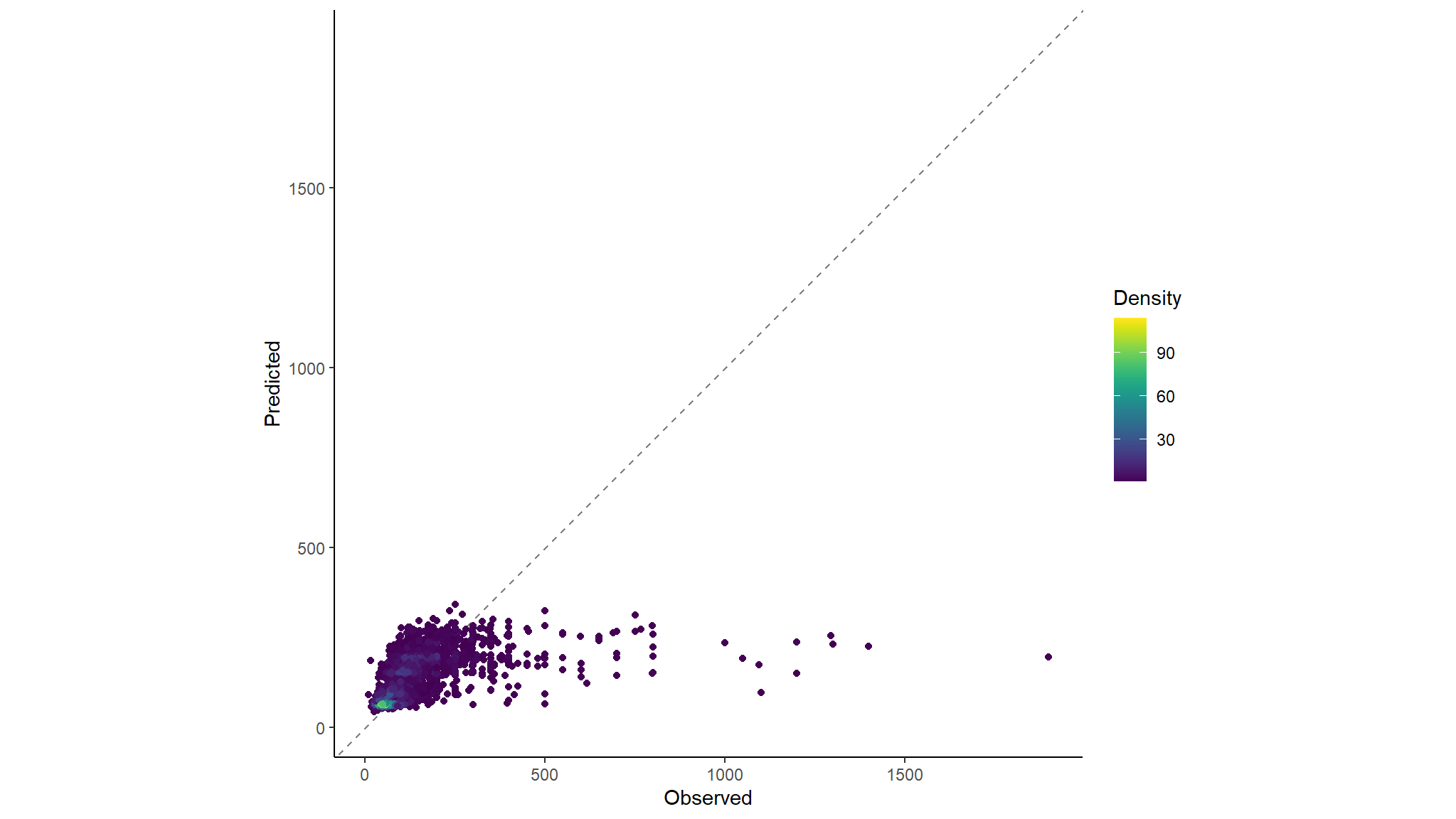

Validation Metric

Earlier, our ‘best’ model produced an rmse of: 108, which is very good and our ensemble model created an rmse of: 108, which is almost identical but just slightly better. This is what ensembling is so often used for; improving an already very good model.

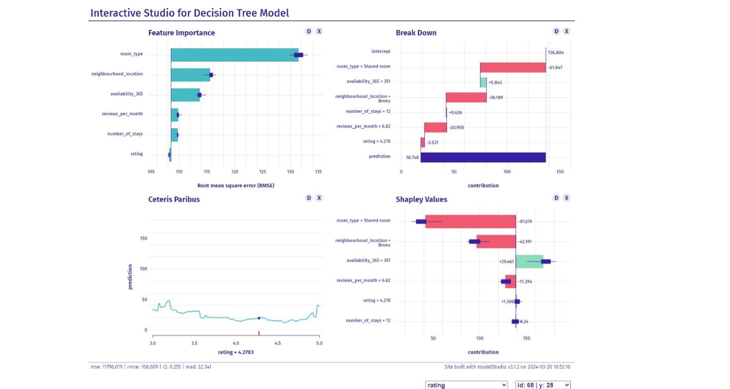
model Explainer


final_fitted <- boosting_test_results |> extract_workflow()


pay_explainer <- DALEXtra::explain_tidymodels(
    final_fitted,
    data    = abnb_test |> select(-price),
    y       = abnb_test$price,
    label="Decision Tree",
    verbose = FALSE

)


# pick observations
new_observation <- abnb_test[1:2,]


# make a studio for the model
modelStudio_obj <- 
    modelStudio::modelStudio(
        explainer       = pay_explainer, 
        viewer          = "browser"
        )


# save the modelstudio object
htmlwidgets::saveWidget(
    widget = modelStudio_obj,
    file   = "model_studio_page.html"
)

Save the model

The model is saved out using the bundle library, which provides a simple and consistent way to prepare R model objects to be saved and re-loaded. This affords users a time saving when saving, sharing and deploying workflows.


# save the model for future use 
model_bundle <- bundle::bundle(final_fitted)
readr::write_rds(model_bundle, file = "model_bundle.rds")