Normal Distribution : Decision Making
Normality
statistics
inference
Decision making
Normal (Gaussian) Random Variable
You have already at least informally seen normal random variables when evaluating linear regression assumptions or perhaps any data analysis procedure . To recall in linear regression , we required responses to be normally distributed at each level of \(X\). Like any continuous random variable, normal (also called Gaussian) random variables have their own pdf, dependent on \(\mu\), the population mean of the variable of interest, and \(\sigma\), the population standard deviation. We find that
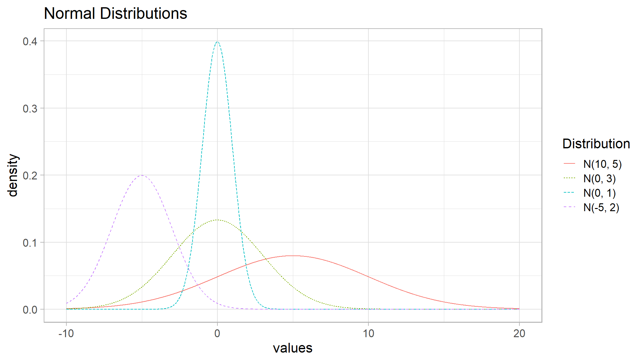
\[\begin{equation} f(y) = \frac{e^{-(y-\mu)^2/ (2 \sigma^2)}}{\sqrt{2\pi\sigma^2}} \quad \textrm{for} \quad -\infty < y < \infty. \end{equation}\]As the parameter names suggest, \(E(Y) = \mu\) and \(SD(Y) = \sigma\). Often, normal distributions are referred to as \(\textrm{N}(\mu, \sigma)\), implying a normal distribution with mean \(\mu\) and standard deviation \(\sigma\). The distribution \(\textrm{N}(0,1)\) is often referred to as the standard normal distribution. A few normal distributions are displayed in Figure below Normal distributions with different values of \(\mu\) and \(\sigma\).
In R, pnorm(y, mean, sd) outputs the probability \(P(Y < y)\) given a mean and standard deviation.
Example: The weight of a box of Fruity Tootie cereal is approximately normally distributed with an average weight of 15 ounces and a standard deviation of 0.5 ounces. What is the probability that the weight of a randomly selected box is more than 15.5 ounces?
Using a normal distribution,
\[\begin{align*} P(Y > 15.5) = \int_{15.5}^{\infty} \frac{e^{-(y-15)^2/ (2\cdot 0.5^2)}}{\sqrt{2\pi\cdot 0.5^2}}dy = 0.159 \end{align*}\]the above formula requires rigorous mathematical transformations and intergrations , that i why we often opt for the
standard Normaldistribution.
Standard Normal distribution
- standardising entails transforming
YintoZsuch that \[Z=\frac{Y-\mu}{\sigma}\] and if that were to happen then the initial formula
\[f(y) = \frac{e^{-(y-\mu)^2/ (2 \sigma^2)}}{\sqrt{2\pi\sigma^2}}\]
transforms to ::
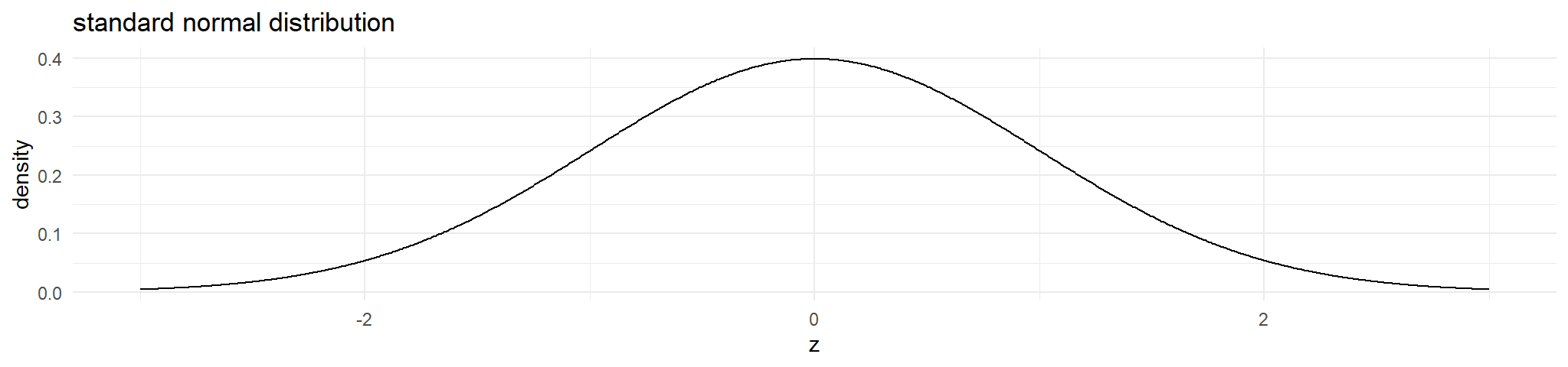
\[\begin{equation} f(z) = \frac{e^{-z^{2}/2}}{\sqrt{2\pi\sigma^2}} \quad \textrm{for} \quad -\infty < z < \infty. \end{equation}\]because \[\frac{(y-\mu)^2}{(\sigma^2)}=z^2\]
standard Normal curve
therefore we would calculate and solve the previous example as follows :
\[P(Y > 15.5)=P(Z> \frac{15.5-15}{0.5})=P(Z> 1)\]
in high school or varsity the above would be found in statistical tables such that \[P(Z>1)=1-P(Z<1)=1-\Phi(1)\]
but it is easier to do in R by using pnorm()
pnorm(1, mean = 0, sd = 1, lower.tail = FALSE)
#> [1] 0.1586553
We can use R with the originial values as well:
pnorm(15.5, mean = 15, sd = 0.5, lower.tail = FALSE)
#> [1] 0.1586553
There is a 16% chance of a randomly selected box weighing more than 15.5 ounces.
example:2 Suppose IQ scores are distributed \(X \sim N\left(100, 16^2\right)\). What is the probability that a randomly selected person’s IQ is less than 90.
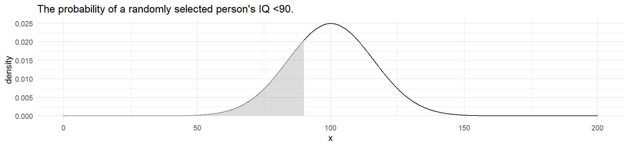
in R
pnorm(q = 90, mean = 100, sd = 16, lower.tail = TRUE)
#> [1] 0.2659855
example 3: What is the probability that a randomly selected person’s IQ is greater than 90
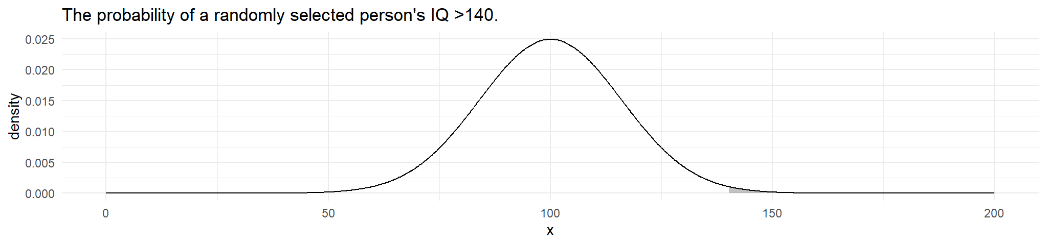
in R
pnorm(q = 140, mean = 100, sd = 16, lower.tail = FALSE)
#> [1] 0.006209665
example 3: What is the probability that a randomly selected person’s IQ is between 92 and 114.
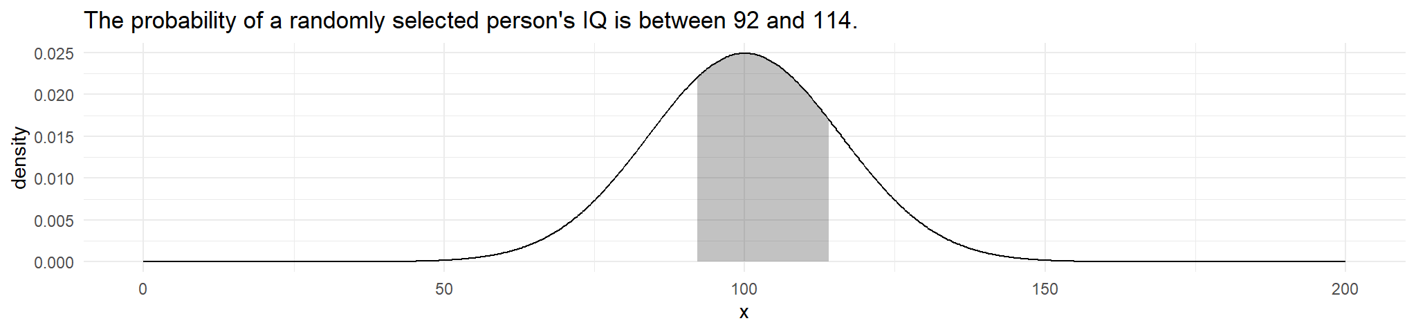
in R
Why do we love the Normal distribution
If has nice properties, such as: if \(X \sim \text{N}(\mu,\sigma^2)\), then \(Z = \displaystyle{{{X - \mu}\over{\sigma}} \sim \text{N}(0,1)}\)
It is a limiting distribution (Central Limit Theorem)
It can be a good approximation for other distributions
We can use R as well:
pnorm(15.5, mean = 15, sd = 0.5, lower.tail = FALSE)
#> [1] 0.1586553
There is a 16% chance of a randomly selected box weighing more than 15.5 ounces.
Summary: Normal distribution
-
notation: \(X \sim \text{N}(\mu,\sigma^2)\)
- range: continuous, all real values
-
distribution: \(f(x) = {{1}\over{\sqrt{2\pi\sigma}}}\exp\left( - {{(x-\mu)^2}\over{2\sigma^2}} \right)\)
- parameters: \(\mu\) the mean and \(\sigma\) the standard deviation
-
mean: \(\mu\)
- variance: \(\sigma^2\)
-
in R:
rnorm,dnorm
A more practical example
- let us examine the following data for
studyhoursandgradesfor a certain class
| StudyHours | Grade |
|---|---|
| 10.00 | 50 |
| 11.50 | 50 |
| 9.00 | 47 |
| 16.00 | 97 |
| 9.25 | 49 |
| 1.00 | 3 |
| 11.50 | 53 |
| 9.00 | 42 |
| 8.50 | 26 |
| 14.50 | 74 |
| 15.50 | 82 |
| 13.75 | 62 |
| 9.00 | 37 |
| 8.00 | 15 |
| 15.50 | 70 |
| 8.00 | 27 |
| 9.00 | 36 |
| 6.00 | 35 |
| 10.00 | 48 |
| 12.00 | 52 |
| 12.50 | 63 |
| 12.00 | 64 |
| 8.00 | NA |
| NA | NA |
Notice that the data are already in tidy format - meaning that:
Each variable is a column
Each observation is a row
Each value is in its own cell
Replace NA in column StudyHours with the mean study hours
df <- df %>%
  mutate(StudyHours = replace_na(StudyHours, mean(StudyHours, na.rm = T)))
Descriptive statistics and data distribution
When examining a variable (for example a sample of student grades), data scientists are particularly interested in its distribution (in other words, how are all the different grade values spread across the sample). The starting point for this exploration is often to visualize the data as a histogram, and see how frequently each value for the variable occurs.
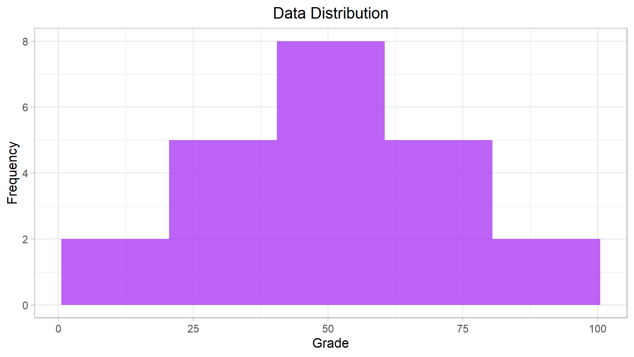
The histogram for grades is a symmetric shape,
What is the Normal distribution saying in its bell shape
- the most frequently occurring grades tend to be in the middle of the range (around 50), with fewer grades at the extreme ends of the scale.
- in essence , unless the teacher is a super teacher , grades close to hundred rarely occur .. less likely that
manystudents would score that much except for a few who are an exception to the rule - again unless the teacher isn`t doing his/her job then few students should fail the test maybe because of less of study
actually that is why the Normal distribution is more common in nature .
- Take a sample of newborn babies , their recorded weight will obviously occur as much , very few would obviously be underweight and very few would be overweight (this is expected if the data was randomly sampled)
- also take a sample of students and measure their IQ , Higher and lower IQ levels are very rare events but still they really occur but not frequently . the list is endless
Measures of central tendency
To understand the distribution better, we can examine so-called measures of central tendency; which is a fancy way of describing statistics that represent the “middle” of the data. The goal of this is to try to find a “typical” value. Common ways to define the middle of the data include:
The
mean: A simple average based on adding together all of the values in the sample set, and then dividing the total by the number of samples.The
median: The value in the middle of the range of all of the sample values.The
mode: The most commonly occuring value in the sample set*.
#> Minimum: 3.00
#> Mean: 49.18
#> Median: 49.50
#> Mode: 50.00
#> Maximum: 97.00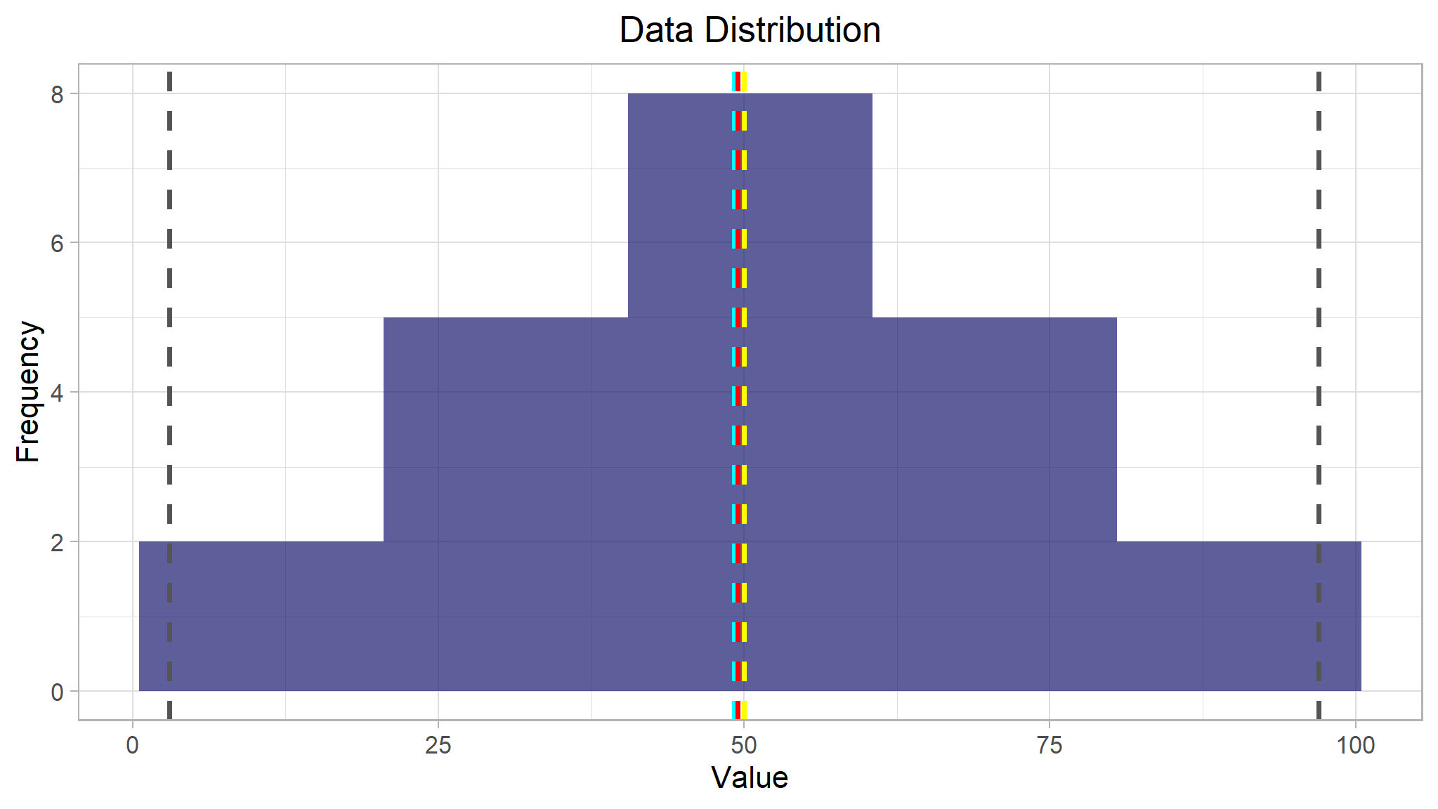
Tip
For the grade data, the mean, median, and mode all seem to be more or less in the middle of the minimum and maximum, at around 50.
Another way to visualize the distribution of a variable is to use a box plot (sometimes called a box-and-whiskers plot). Let’s create one for the grade data.
# Get the variable to examine
var <- df %>% select(Grade)

# Plot a box plot
var %>%
  ggplot(aes(x = 1, y = Grade))+
  geom_boxplot(fill = "#E69F00", color = "gray23", alpha = 0.7)+
# Add titles and labels
  ggtitle("Data Distribution")+
  xlab("")+
  ylab("Grade")+
  theme(plot.title = element_text(hjust = 0.5))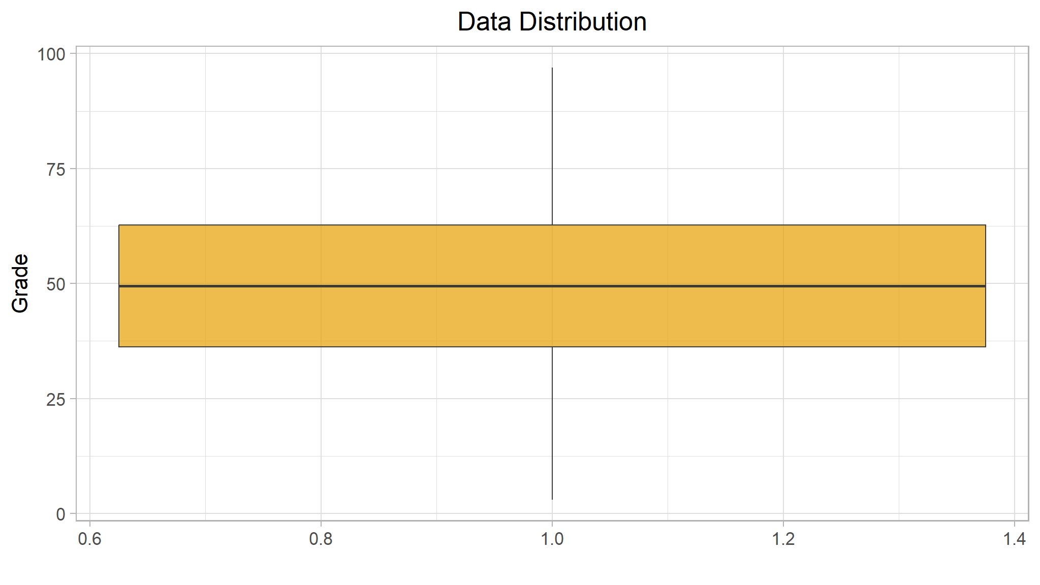
Note
The box plot shows the distribution of the grade values in a different format to the histogram. The box part of the plot shows where the inner two quartiles of the data reside - so in this case, half of the grades are between approximately 36 and 63. The whiskers extending from the box show the outer two quartiles; so the other half of the grades in this case are between 0 and 36 or 63 and 100. The line in the box indicates the median value.
Combine the results
#> [[1]]
#> Minimum: 3.00
#> Mean: 49.18
#> Median: 49.50
#> Mode: 50.00
#> Maximum: 97.00
#>
#> [[2]]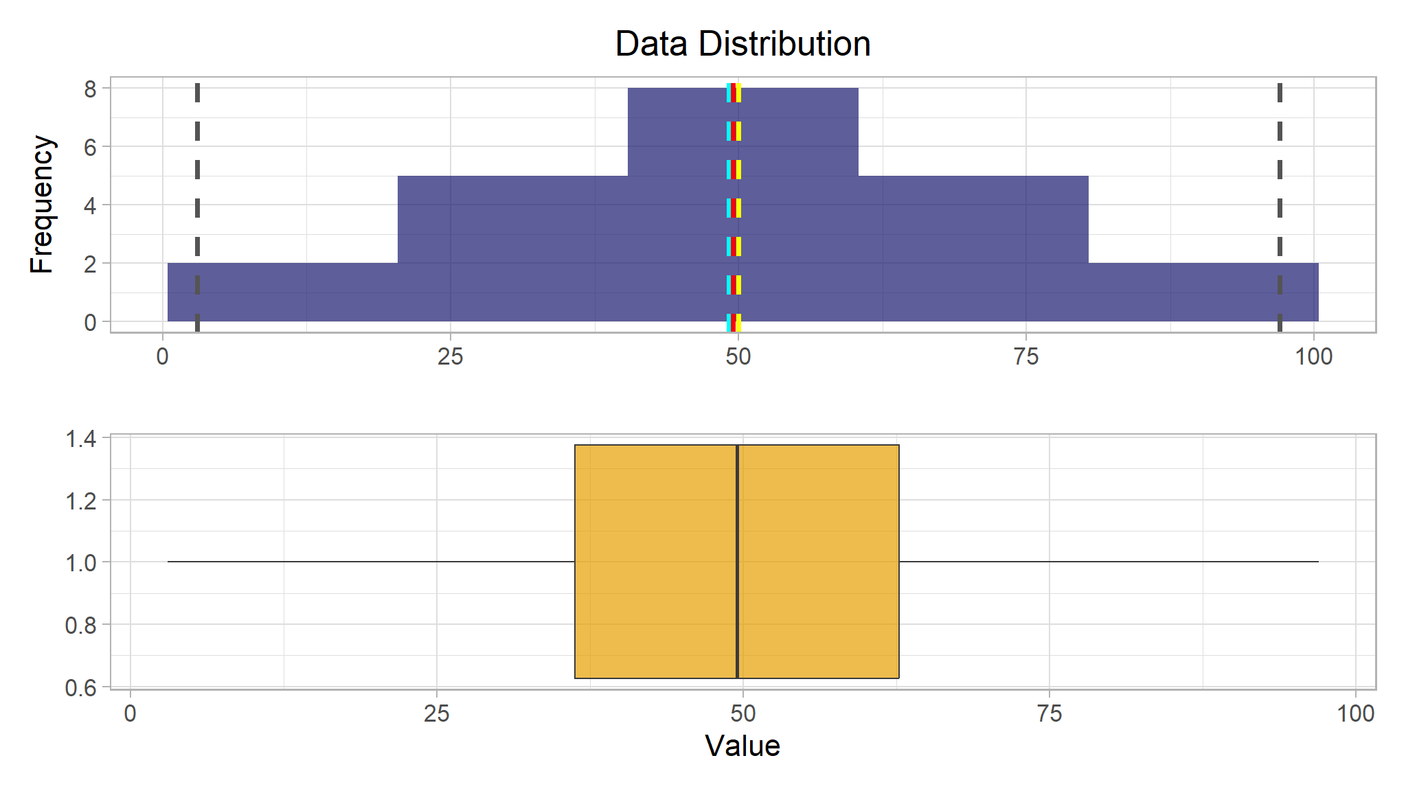
Note
All of the measurements of central tendency are right in the middle of the data distribution, which is symmetric with values becoming progressively lower in both directions from the middle.
Density plots are more easy to read
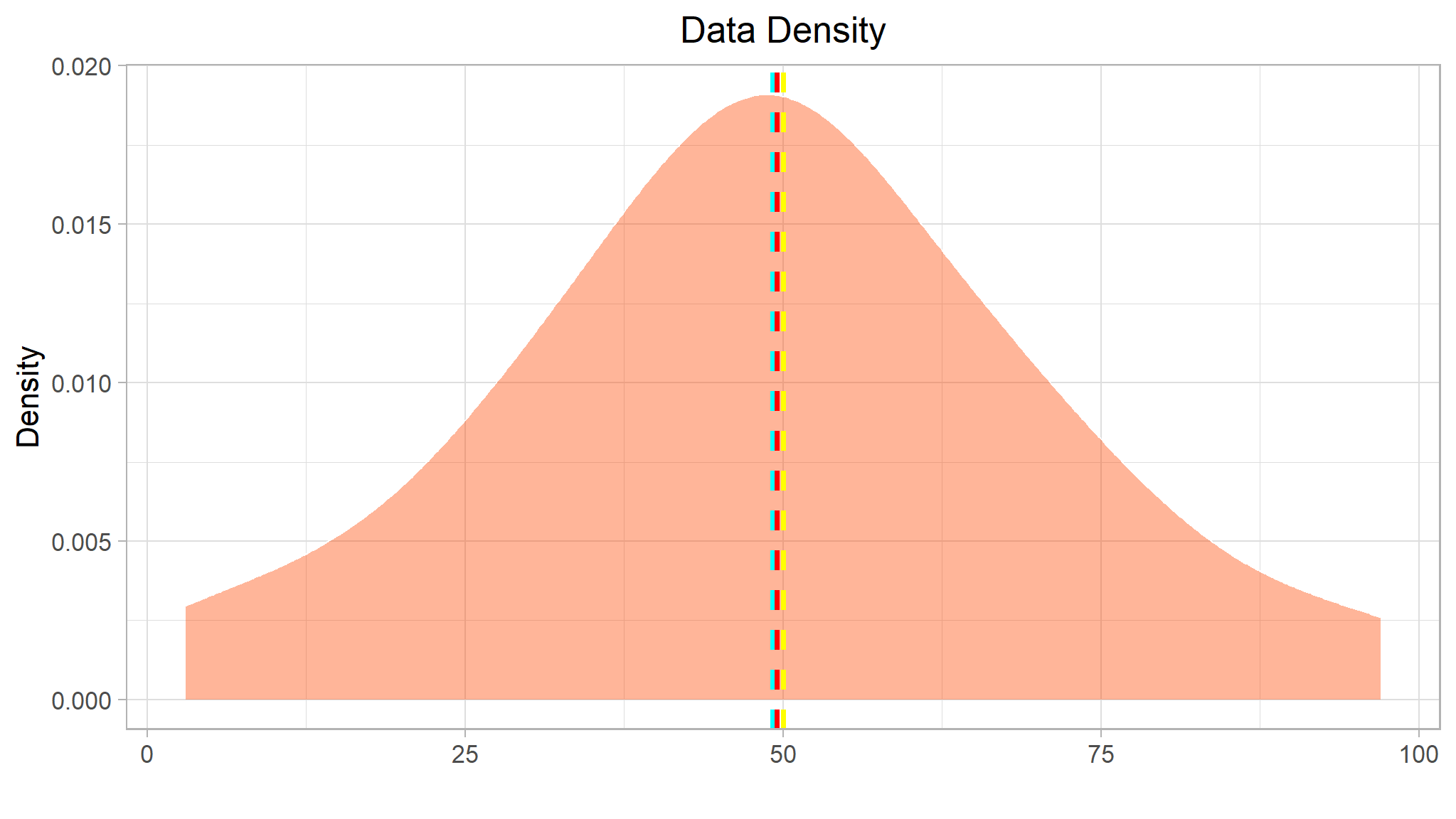
Note
As expected from the histogram of the sample, the density of the Grade column shows the characteristic ’bell curve” of what statisticians call a normal distribution with the mean and mode at the center and symmetric tails.
Measures of variance
So now we have a good idea where the middle of the grade and study hours data distributions are. However, there’s another aspect of the distributions we should examine: how much variability is there in the data?
Typical statistics that measure variability in the data include:
*Range*: The difference between the maximum and minimum. There’s no built-in function for this, but it’s easy to calculate using the*min*and*max*functions. Another approach would be to use Base R’sbase::range()which returns a vector containing theminimumandmaximumof all the given arguments. Wrapping this inbase::diff()will get you well on your way to finding the range.*Variance*: The average of the squared difference from the mean. You can use the built-in*var*function to find this.*Standard Deviation*: The square root of the variance. You can use the built-in*sd*function to find this.
#> $Grade
#> - Range: 94.00
#> - Variance : 472.54
#> - Std.Dev : 21.74
#>
#> $StudyHours
#> - Range: 15.00
#> - Variance : 12.16
#> - Std.Dev : 3.49
Of these statistics, the standard deviation is generally the most useful. It provides a measure of variance in the data on the same scale as the data itself (so grade points for the Grade distribution and hours for the StudyHours distribution). The higher the standard deviation, the more variance there is when comparing values in the distribution to the distribution mean - in other words, the data is more spread out.
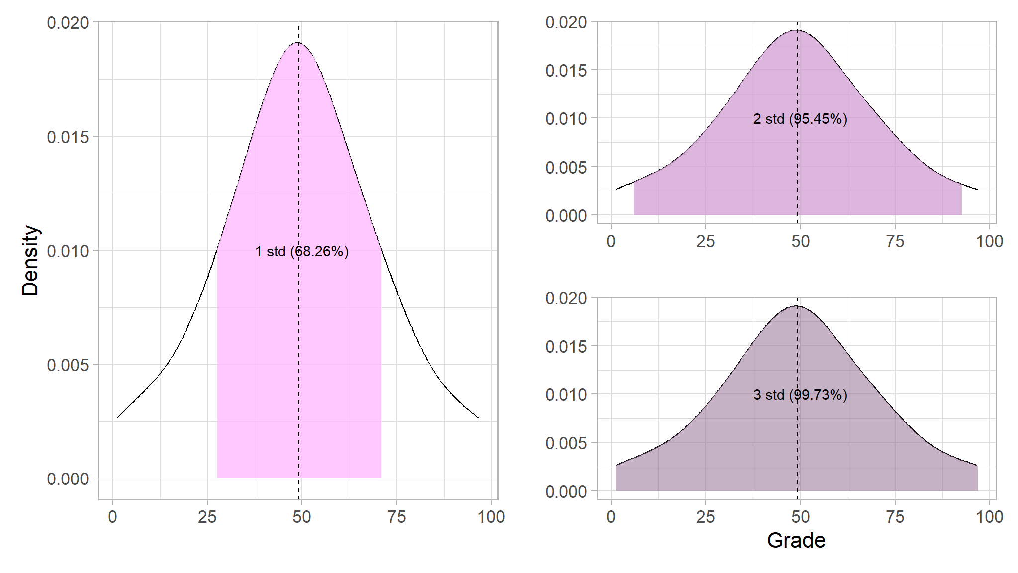
When working with a normal distribution, the standard deviation works with the particular characteristics of a normal distribution to provide even greater insight. This can be summarized using the 68–95–99.7 rule, also known as the empirical rulewhich is described as follows:
Note
In any normal distribution:
Approximately 68.26% of values fall within one standard deviation from the mean.
Approximately 95.45% of values fall within two standard deviations from the mean.
Approximately 99.73% of values fall within three standard deviations from the mean.
# Get the variable to examine
col <- df['Grade']

# Get the mean
me_an <- mean(pull(col))

# Get the standard deviation
st_dev <- sd(pull(col))

# Find proportion that will fall within 1 standard deviation
one_st_dev <- pnorm((me_an + st_dev), mean = me_an, sd = st_dev) -
  pnorm((me_an - st_dev), mean = me_an, sd = st_dev)

# Find proportion that will fall within 2 standard deviation
two_st_dev <- pnorm((me_an + (2*st_dev)), mean = me_an, sd = st_dev) -
  pnorm((me_an - (2*st_dev)), mean = me_an, sd = st_dev)

# Find proportion that will fall within 3 standard deviation
three_st_dev <- pnorm((me_an + (3*st_dev)), mean = me_an, sd = st_dev) -
  pnorm((me_an - (3*st_dev)), mean = me_an, sd = st_dev)

glue::glue(
  '
  {format(round(one_st_dev*100, 2), nsmall = 2)}% of grades fall within one standard deviation from the mean.
  {format(round(two_st_dev*100, 2), nsmall = 2)}% of grades fall within two standard deviation from the mean.
  {format(round(three_st_dev*100, 2), nsmall = 2)}% of grades fall within three standard deviation from the mean.

  '
)
#> 68.27% of grades fall within one standard deviation from the mean.
#> 95.45% of grades fall within two standard deviation from the mean.
#> 99.73% of grades fall within three standard deviation from the mean.
Note
There is no doubt that the distribution of grades indeed follows a normal distribution!
Note
Since we know that the mean grade is 49.18, the standard deviation is 21.74, and distribution of grades is normal; we can calculate that 68.26% of students should achieve a grade between 27.44 and 70.92 as shown in the first plot above.
The descriptive statistics we’ve used to understand the distribution of the student data variables are the basis of statistical analysis.