Introduction to Customer Churning

Comparing R and Powerbi DAX

Note

• this blog aims to compare how things are done in R and Powerbi

Data Analysis Expressions (DAX) is a formula expression language used in Analysis Services, Power BI, and Power Pivot in Excel. DAX formulas include functions, operators, and values to perform advanced calculations and queries on data in related tables and columns in tabular data models.

• This article provides only a basic introduction to the most important concepts in DAX while comparing them to R

library(tidyverse)

churn<-readr::read_csv("Databel_Data.csv")
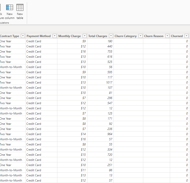
churn |> 
  head(10) |> 
  flextable::flextable()

Customer ID	Churn Label	Account Length (in months)	Local Calls	Local Mins	Intl Calls	Intl Mins	Intl Active	Intl Plan	Extra International Charges	Customer Service Calls	Avg Monthly GB Download	Unlimited Data Plan	Extra Data Charges	State	Phone Number	Gender	Age	Under 30	Senior	Group	Number of Customers in Group	Device Protection & Online Backup	Contract Type	Payment Method	Monthly Charge	Total Charges	Churn Category	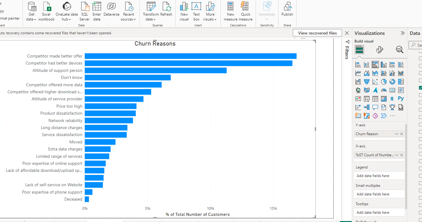Churn Reason
4444-BZPU	No	1	3	8.0	0	0.0	No	no	0	0	3	Yes	0	KS	382-4657	Female	35	No	No	No	0	No	Month-to-Month	Direct Debit	10	10
5676-PTZX	No	33	179	431.3	0	0.0	No	no	0	0	3	Yes	0	OH	371-7191	Male	49	No	No	No	0	Yes	One Year	Paper Check	21	703
8532-ZEKQ	No	44	82	217.6	0	0.0	No	yes	0	0	3	Yes	0	OH	375-9999	Male	51	No	No	No	0	Yes	One Year	Direct Debit	23	1,014
1314-SMPJ	No	10	47	111.6	60	71.0	Yes	yes	0	0	2	Yes	0	MO	329-9001	Female	41	No	No	No	0	No	Month-to-Month	Paper Check	17	177
2956-TXCJ	No	62	184	621.2	310	694.4	Yes	yes	0	0	3	Yes	0	WV	330-8173	Male	51	No	No	No	0	No	One Year	Direct Debit	28	1,720
9152-DEPY	No	17	68	120.7	0	0.0	No	no	0	0	0	No	0	RI	344-9403	Male	23	Yes	No	No	0	No	Two Year	Credit Card	9	156
1958-SDSO	No	57	428	849.2	0	0.0	No	no	0	0	5	Yes	0	IA	363-1107	Male	38	No	No	No	0	Yes	One Year	Credit Card	47	2,671
8787-QZUC	No	25	54	203.7	0	0.0	No	no	0	0	12	Yes	0	IA	366-9238	Male	29	Yes	No	No	0	Yes	Month-to-Month	Direct Debit	47	1,197
7768-OQJE	No	70	171	627.4	0	0.0	No	no	0	0	1	Yes	0	NY	351-7269	Female	47	No	No	No	0	Yes	Two Year	Credit Card	52	3,593
7716-RHEB	No	50	206	445.8	0	0.0	No	no	0	0	0	No	0	ID	350-8884	Female	61	No	No	No	0	No	One Year	Paper Check	11	539

Data exploration

Note

• before any analysis , it is mandatory to learn more about the rows in our data
• things like the number of rows in our data and duplicate columns in our data are very important to understand

COUNT : R

churn |> 
  summarise(`number of customers` = n(),
            `distinct customers` = n_distinct(`Customer ID`))

# A tibble: 1 × 2
  `number of customers` `distinct customers`
                  <int>                <int>
1                  6687                 6687

OR

(`Number of Customers` <- count(churn))

# A tibble: 1 × 1
      n
  <int>
1  6687

COUNT : DAX

Note

• in powerbi our dataframe is Databel - Data and to index our data we use 'Databel - Data'[variable]

to find the number of rows we use COUNT() or COUNTROWS()

Number of Customers = COUNT('Databel - Data'[Customer ID])

to find the number of UNIQUE customers we use DISTINCTCOUNT() or COUNTROWS()

Number of Customers = DISTINCTCOUNT('Databel - Data'[Customer ID])

Data manipulation

IF STATEMENTS

IF statements : R

in dplyr we use ifelse() in conjuction with mutate() to create a new variable based on a certain condition or criteria

(churn <- churn |> 
   mutate(churned = ifelse(`Churn Label` == "Yes",1,0)) |> 
   relocate(churned))

# A tibble: 6,687 × 30
   churned `Customer ID` `Churn Label` Account Length (in months…¹ `Local Calls`
     <dbl> <chr>         <chr>                               <dbl>         <dbl>
 1       0 4444-BZPU     No                                      1             3
 2       0 5676-PTZX     No                                     33           179
 3       0 8532-ZEKQ     No                                     44            82
 4       0 1314-SMPJ     No                                     10            47
 5       0 2956-TXCJ     No                                     62           184
 6       0 9152-DEPY     No                                     17            68
 7       0 1958-SDSO     No                                     57           428
 8       0 8787-QZUC     No                                     25            54
 9       0 7768-OQJE     No                                     70           171
10       0 7716-RHEB     No                                     50           206
# ℹ 6,677 more rows
# ℹ abbreviated name: ¹​`Account Length (in months)`
# ℹ 25 more variables: `Local Mins` <dbl>, `Intl Calls` <dbl>,
#   `Intl Mins` <dbl>, `Intl Active` <chr>, `Intl Plan` <chr>,
#   `Extra International Charges` <dbl>, `Customer Service Calls` <dbl>,
#   `Avg Monthly GB Download` <dbl>, `Unlimited Data Plan` <chr>,
#   `Extra Data Charges` <dbl>, State <chr>, `Phone Number` <chr>, …

IF statements : DAX

in DAX we use IF() , uses the same idea as R

Churned = IF('Databel - Data'[Churn Label]="Yes",1,0)

Calculate churn Rate

for that we first calculate the number of customers that churned ,

In R

• in R we can sum over the churned column since we know it contains Zeros and ones

(`Number of Churned Customers` = sum(churn$churned))

[1] 1796

• about 1796 people churned

In DAX

do it in DAX , we use sum() or SUM() just like R

The only difference is we used $ in R

Number of Churned Customers = SUM('Databel - Data'[Churned])

now determine the churn rate in R

(`Churn Rate` = `Number of Churned Customers`/`Number of Customers`$n)* 100

[1] 26.85808

churn rate in DAX

Churn Rate in PowerBi , just like in R we use / to imply divide

Churn Rate = [Number of Churned Customers]/[Number of Customers]

overally we get 26.86% churn rate

Lets determine the frequent reasaons for churning

In R

in R we use ggplot2 package to plot our data

churn |>
  na.omit() |> 
  group_by(`Churn Reason`) |> 
  summarise(n = n()) |> 
  ggplot(aes(x= fct_reorder(`Churn Reason`,n) , y= n))+
  geom_col(fill="blue")+
  coord_flip()+
  ggthemes::theme_economist()+
  labs(x="Churn Reason",y="number of customers")

In Powerbi

in Powerbi we simply selected a clustered bar chart

More advanced data manipulation

table(churn$`Contract Type`)

Month-to-Month       One Year       Two Year 
          3411           1479           1797 

suppose we intend to have just year and Monthly contract types , we can choose to bundle up One year and Two Year into just Year category.

in R we can use case_when()

(churn<-churn |> 
   mutate(`Contract Category` = case_when(`Contract Type` =="One Year"~ "Yearly",
                                          `Contract Type` =="Two Year"~ "Yearly",
                                          `Contract Type` =="Month-to-Month"~ "Monthly")) |> 
  relocate(`Contract Category`))

# A tibble: 6,687 × 31
   `Contract Category` churned `Customer ID` `Churn Label`
   <chr>                 <dbl> <chr>         <chr>        
 1 Monthly                   0 4444-BZPU     No           
 2 Yearly                    0 5676-PTZX     No           
 3 Yearly                    0 8532-ZEKQ     No           
 4 Monthly                   0 1314-SMPJ     No           
 5 Yearly                    0 2956-TXCJ     No           
 6 Yearly                    0 9152-DEPY     No           
 7 Yearly                    0 1958-SDSO     No           
 8 Monthly                   0 8787-QZUC     No           
 9 Yearly                    0 7768-OQJE     No           
10 Yearly                    0 7716-RHEB     No           
# ℹ 6,677 more rows
# ℹ 27 more variables: `Account Length (in months)` <dbl>, `Local Calls` <dbl>,
#   `Local Mins` <dbl>, `Intl Calls` <dbl>, `Intl Mins` <dbl>,
#   `Intl Active` <chr>, `Intl Plan` <chr>,
#   `Extra International Charges` <dbl>, `Customer Service Calls` <dbl>,
#   `Avg Monthly GB Download` <dbl>, `Unlimited Data Plan` <chr>,
#   `Extra Data Charges` <dbl>, State <chr>, `Phone Number` <chr>, …

in powerbi we use SWITCH()

SWITCH(<expression>, <value>, <result>[, <value>, <result>]…[, <else>])

Contract Category = SWITCH('Databel - Data'[Contract Type], 
                           "One Year", "Yearly", 
                           "Two Year", "Yearly", 
                           "Monthly")

Churn Rates By state

R

In R we use the power of mutate and sprintf()

churn |> 
  group_by(State) |> 
  summarise(`# of customers` = n(),
            `# of churned customers` = sum(churned),
            `Churn Rate` = sprintf("%.2f%%",`# of churned customers`/`# of customers`* 100)) |> 
  knitr::kable()

State	# of customers	# of churned customers	Churn Rate
AK	104	30	28.85%
AL	161	46	28.57%
AR	110	27	24.55%
AZ	128	30	23.44%
CA	68	43	63.24%
CO	132	29	21.97%
CT	148	38	25.68%
DC	108	21	19.44%
DE	122	37	30.33%
FL	127	27	21.26%
GA	108	25	23.15%
HI	106	28	26.42%
IA	90	24	26.67%
ID	147	41	27.89%
IL	116	33	28.45%
IN	143	42	29.37%
KS	141	36	25.53%
KY	118	36	30.51%
LA	103	25	24.27%
MA	131	33	25.19%
MD	140	46	32.86%
ME	124	29	23.39%
MI	146	40	27.40%
MN	168	38	22.62%
MO	127	36	28.35%
MS	130	37	28.46%
MT	137	43	31.39%
NC	136	28	20.59%
ND	124	31	25.00%
NE	122	40	32.79%
NH	112	36	32.14%
NJ	137	37	27.01%
NM	124	30	24.19%
NV	132	36	27.27%
NY	167	39	23.35%
OH	158	55	34.81%
OK	123	24	19.51%
OR	156	48	30.77%
PA	90	30	33.33%
RI	131	33	25.19%
SC	120	36	30.00%
SD	120	27	22.50%
TN	106	24	22.64%
TX	145	42	28.97%
UT	144	36	25.00%
VA	155	42	27.10%
VT	147	39	26.53%
WA	132	29	21.97%
WI	156	39	25.00%
WV	213	57	26.76%
WY	154	38	24.68%

Powerbi

in powerbi we use a table to summarise our data just by clicking

Filtering

• filtering is a common pocedure in data science

here is how we do it in R as compared to DAX

In filter and average in R

• In R we use filter() then summarise() to get the mean for only a certain category

churn |> 
  filter(`Payment Method` == "Direct Debit") |> 
  summarise(`avg total charges in direct debit` = mean(`Monthly Charge`))

# A tibble: 1 × 1
  `avg total charges in direct debit`
                                <dbl>
1                                35.1

filter and Average In DAX

CALCULATE(<expression>[, <filter1> [, <filter2> [, …]]])

avg total charges in direct debit = CALCULATE(AVERAGE('Databel - Data'[Monthly Charge]),
                                              'Databel - Data'[Payment Method]="Direct Debit")

filter and COUNT in R

churn |> 
  filter(`Payment Method` == "Direct Debit") |> 
  summarise(`count customers in direct Debit` = n_distinct(`Customer ID`))

# A tibble: 1 × 1
  `count customers in direct Debit`
                              <int>
1                              3702

filter and COUNT in DAX

avg total charges in direct debit = CALCULATE(DISTINCTCOUNT('Databel - Data'[CUSTOMER ID]),
                                              'Databel - Data'[Payment Method]="Direct Debit")