Probability Distributions to ACE your CS1 EXAM

An R interactive learning (STATSPYSCHICS.COM)

Author

Bongani Ncube

Published

5 March 2026

Warning: package 'ggplot2' was built under R version 4.3.3

Note

by the end of this tutorial you will be able to answer these IFOA questions

Mathematical Representations of Distributions

Review of mentioned random variables.
Distribution Name	pmf / pdf	Parameters	Possible Y Values	Description
Binomial	${n \choose y} p^y (1-p)^{n-y}$	$p,\ n$	$0, 1, \ldots , n$	Number of successes after $n$ trials
Geometric	$(1-p)^yp$	$p$	$0, 1, \ldots, \infty$	Number of failures until the first success
Negative Binomial	${y + r - 1\choose r-1} (1-p)^{y}(p)^r$	$p,\ r$	$0, 1, \ldots, \infty$	Number of failures before $r$ successes
Hypergeometric	${m \choose y}{N-m \choose n-y}\big/{N \choose n}$	$n,\ m,\ N$	$0, 1, \ldots , \min(m,n)$	Number of successes after $n$ trials without replacement
Poisson	${e^{-\lambda}\lambda^y}\big/{y!}$	$\lambda$	$0, 1, \ldots, \infty$	Number of events in a fixed interval
Exponential	$\lambda e^{-\lambda y}$	$\lambda$	$(0, \infty)$	Wait time for one event in a Poisson process
Gamma	$\displaystyle\frac{\lambda^r}{\Gamma(r)} y^{r-1} e^{-\lambda y}$	$\lambda, \ r$	$(0, \infty)$	Wait time for $r$ events in a Poisson process
Normal	$\displaystyle\frac{e^{-(y-\mu)^2/ (2 \sigma^2)}}{\sqrt{2\pi\sigma^2}}$	$\mu,\ \sigma$	$(-\infty,\ \infty)$	Used to model many naturally occurring phenomena
Beta	$\frac{\Gamma(\alpha + \beta)}{\Gamma(\alpha)\Gamma(\beta)} y^{\alpha-1} (1-y)^{\beta-1}$	$\alpha,\ \beta$	$(0,\ 1)$	Useful for modeling probabilities

Probability distributions in R

R has four common funtions for working with probability distributions which are ::

d__ gives the density of the distribution at a value $x$
p__ gives $P(X \leq x)$ with lower.tail = TRUE OR $P(X>x)$ otherwise

this is, the probability of a variable X taking a value lower than 𝑥

q__ gives quantiles , so the value of x such that $F(x) = p$
r__ gives random deviates of the specified distribution

Discrete Random Variables

A discrete random variable has a countable number of possible values; for example, we may want to measure the number of people in a household or the number of crimes committed on a college campus. With discrete random variables, the associated probabilities can be calculated for each possible value using a probability mass function (pmf).

A discrete random variable $X$ is described by its probability mass function $f(x) = P(X = x)$. The set of $x$ values for which $f(x) > 0$ is called the support. If the distribution depends on unknown parameter(s) $\theta$ we write it as $f(x; \theta)$ (frequentist) or $f(x | \theta)$ (Bayesian).

Binary Random Variable

Consider the event of flipping a (possibly unfair) coin. If the coin lands heads, let’s consider this a success and record $Y = 1$. A series of these events is a Bernoulli process, independent trials that take on one of two values (e.g., 0 or 1). These values are often referred to as a failure and a success, and the probability of success is identical for each trial. Suppose we only flip the coin once, so we only have one parameter, the probability of flipping heads, $p$. If we know this value, we can express $P(Y=1) = p$ and $P(Y=0) = 1-p$. In general, if we have a Bernoulli process with only one trial, we have a binary distribution (also called a Bernoulli distribution) where

\[\begin{equation} P(Y = y) = p^y(1-p)^{1-y} \quad \textrm{for} \quad y = 0, 1. (\#eq:binaryRV) \end{equation}\] If $Y \sim \textrm{Binary}(p)$, then $Y$ has mean $E(Y) = p$ and standard deviation $SD(Y) = \sqrt{p(1-p)}$.

Example 1: Your playlist of 200 songs has 5 which you cannot stand. What is the probability that when you hit shuffle, a song you tolerate comes on?

Assuming all songs have equal odds of playing, we can calculate $p = \frac{200-5}{200} = 0.975$, so there is a 97.5% chance of a song you tolerate playing, since $P(Y=1)=.975^1*(1-.975)^0$.

Summary

A discrete random variable $Y$ is described by its probability mass function $f(y) = P(X = y)$. The set of $y$ values for which $f(y) > 0$ is called the support. If the distribution depends on unknown parameter(s) $\theta$ we write it as $f(y; \theta)$ (frequentist) or $f(y | \theta)$ (Bayesian).

Binomial Random Variable

Suppose we flipped an unfair coin $n$ times and recorded $Y$, the number of heads after $n$ flips. If we consider a case where $p = 0.25$ and $n = 4$, then here $P(Y=0)$ represents the probability of no successes in 4 trials, i.e., 4 consecutive failures. The probability of 4 consecutive failures is $P(Y = 0) = P(TTTT) = (1-p)^4 = 0.75^4$. When we consider $P(Y = 1)$, we are interested in the probability of exactly 1 success anywhere among the 4 trials. There are $\binom{4}{1} = 4$ ways to have exactly 1 success in 4 trials, so $P(Y = 1) = \binom{4}{1}p^1(1-p)^{4-1} = (4)(0.25)(0.75)^3$. In general, if we carry out a sequence of $n$ Bernoulli trials (with probability of success $p$) and record $Y$, the total number of successes, then $Y$ follows a binomial distribution, where

\[\begin{equation} P(Y=y) = \binom{n}{y} p^y (1-p)^{n-y} \quad \textrm{for} \quad y = 0, 1, \ldots, n. (\#eq:binomRV) \end{equation}\] If $Y \sim \textrm{Binomial}(n,p)$, then $E(Y) = np$ and $SD(Y) = \sqrt{np(1-p)}$. On the left side $n$ remains constant. We see that as $p$ increases, the center of the distribution ($E(Y) = np$) shifts right. On the right, $p$ is held constant. As $n$ increases, the distribution becomes less skewed.

Binomial distributions with different values of $n$ and $p$.

Note that if $n=1$,

\[\begin{align*} P(Y=y) &= \binom{1}{y} p^y(1-p)^{1-y} \\ &= p^y(1-p)^{1-y}\quad \textrm{for}\quad y = 0, 1, \end{align*}\] a Bernoulli distribution! In fact, Bernoulli random variables are a special case of binomial random variables where $n=1$.

In R we can use the function dbinom(y, n, p), which outputs the probability of $y$ successes given $n$ trials with probability $p$, i.e., $P(Y=y)$ for $Y \sim \textrm{Binomial}(n,p)$.

Example 2: While taking a multiple choice test, a student encountered 10 problems where she ended up completely guessing, randomly selecting one of the four options. What is the chance that she got exactly 2 of the 10 correct?

Knowing that the student randomly selected her answers, we assume she has a 25% chance of a correct response. Thus, $P(Y=2) = {10 \choose 2}(.25)^2(.75)^8 = 0.282$. We can use R to verify this:

Therefore, there is a 28% chance of exactly 2 correct answers out of 10.

Continuous Random Variables

A continuous random variable can take on an uncountably infinite number of values. With continuous random variables, we define probabilities using probability density functions (pdfs). Probabilities are calculated by computing the area under the density curve over the interval of interest. So, given a pdf, $f(y)$, we can compute

\[\begin{align*} P(a \le Y \le b) = \int_a^b f(y)dy. \end{align*}\] This hints at a few properties of continuous random variables:

$\int_{-\infty}^{\infty} f(y)dy = 1$.
For any value $y$, $P(Y = y) = \int_y^y f(y)dy = 0$.
Because of the above property, $P(y < Y) = P(y \le Y)$. We will typically use the first notation rather than the second, but both are equally valid.

Exponential Random Variable

Suppose we have a Poisson process with rate $\lambda$, and we wish to model the wait time $Y$ until the first event. We could model $Y$ using an exponential distribution, where

\[\begin{equation} f(y) = \lambda e^{-\lambda y} \quad \textrm{for} \quad y > 0 \end{equation}\] where $E(Y) = 1/\lambda$ and $SD(Y) = 1/\lambda$. As $\lambda$ increases, $E(Y)$ tends towards 0, and distributions “die off” quicker.

Exponential distributions with $\lambda = 0.5, 1,$ and $5$.

If we wish to use R, pexp(y, lambda) outputs the probability $P(Y < y)$ given $\lambda$.

Example 7: Refer to Example 6. What is the probability that 10 days or fewer elapse between two tickets being issued?

We know the town’s police issue 5 tickets per month. For simplicity’s sake, assume each month has 30 days. Then, the town issues $\frac{1}{6}$ tickets per day. That is $\lambda = \frac{1}{6}$, and the average wait time between tickets is $\frac{1}{1/6} = 6$ days. Therefore,

\[\begin{align*} P(Y < 10) = \int_{0}^{10} \textstyle \frac16 e^{-\frac16y} dy = 0.81. \end{align*}\]

We can also use R:

Hence, there is a 81% chance of waiting fewer than 10 days between tickets.

Gamma Random Variable

Once again consider a Poisson process. When discussing exponential random variables, we modeled the wait time before one event occurred. If $Y$ represents the wait time before $r$ events occur in a Poisson process with rate $\lambda$, $Y$ follows a gamma distribution where

\[\begin{equation} f(y) = \frac{\lambda^r}{\Gamma(r)} y^{r-1} e^{-\lambda y}\quad \textrm{for} \quad y >0. (\#eq:gammaRV) \end{equation}\]

If $Y \sim \textrm{Gamma}(r, \lambda)$ then $E(Y) = r/\lambda$ and $SD(Y) = \sqrt{r/\lambda^2}$. Observe that means increase as $r$ increases, but decrease as $\lambda$ increases.

Gamma distributions with different values of $r$ and $\lambda$.

x <- seq(0, 7, by = 0.01)
`r = 1, lambda = 1` <- dgamma(x, 1, rate = 1)
`r = 2, lambda = 1` <- dgamma(x, 2, rate = 1) 
`r = 5, lambda = 5` <- dgamma(x, 5, rate = 5)
`r = 5, lambda = 7` <- dgamma(x, 5, rate = 7)

gammaDf <- tibble(x, `r = 1, lambda = 1`, `r = 2, lambda = 1`, `r = 5, lambda = 5`, `r = 5, lambda = 7`) %>%
  gather(2:5, key = "Distribution", value = "value") %>%
  mutate(Distribution = factor(Distribution, 
                               levels = c("r = 2, lambda = 1", 
                                          "r = 1, lambda = 1", 
                                          "r = 5, lambda = 5", 
                                          "r = 5, lambda = 7")))

ggplot(data = gammaDf, aes(x = x, y = value, 
                           color = Distribution)) +
  geom_line(aes(linetype = Distribution)) +
  xlab("values") + ylab("density") + 
  labs(title = "Gamma Distributions") +
  theme(legend.title = element_blank())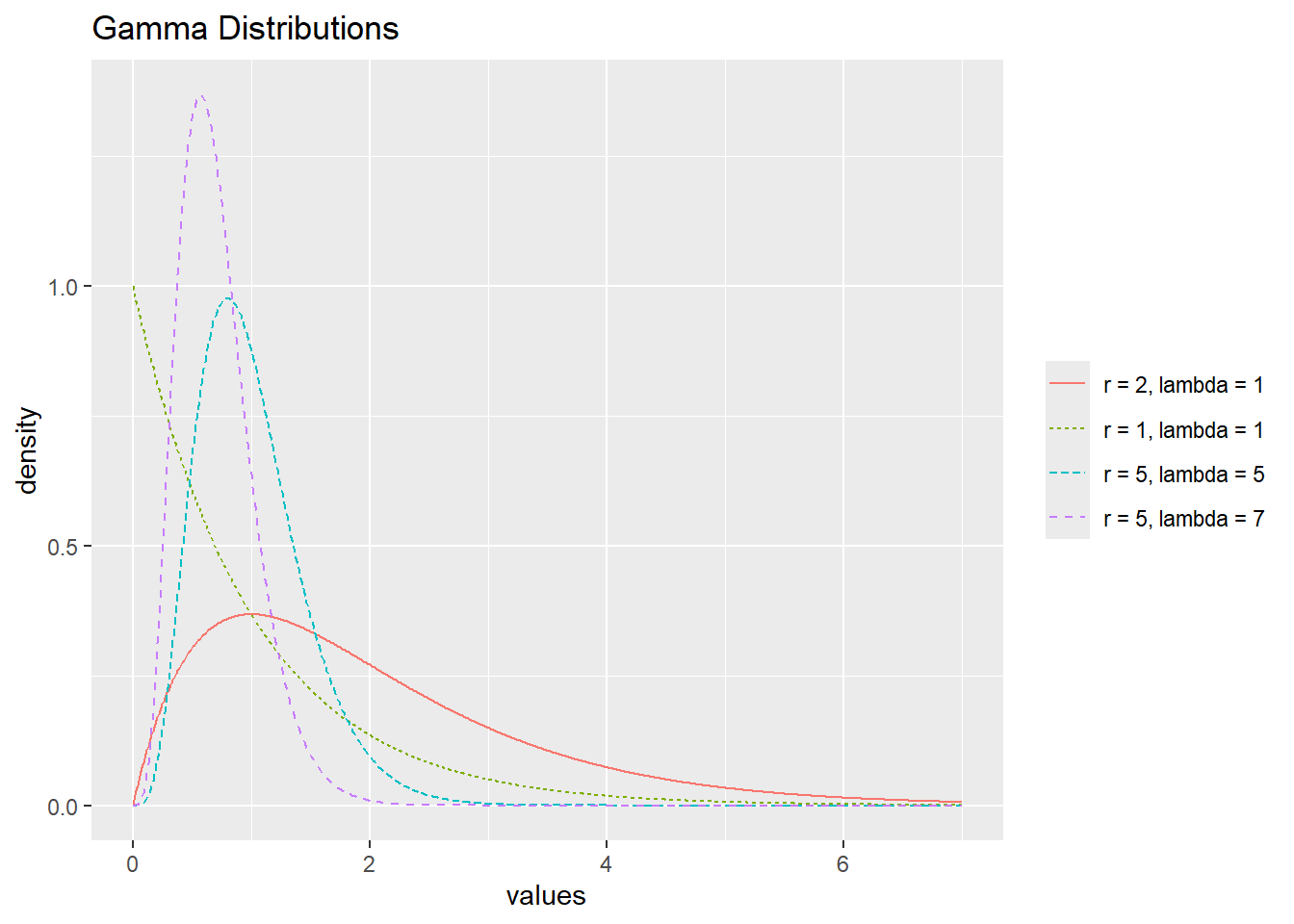

Note that if we let $r = 1$, we have the following pdf,

\[\begin{align*} f(y) &= \frac{\lambda}{\Gamma(1)} y^{1-1} e^{-\lambda y} \\ &= \lambda e^{-\lambda y} \quad \textrm{for} \quad y > 0, \end{align*}\] an exponential distribution. Just as how the geometric distribution was a special case of the negative binomial, exponential distributions are in fact a special case of gamma distributions!

Just like negative binomial, the pdf of a gamma distribution is defined for all real, non-negative $r$.

In R, pgamma(y, r, lambda) outputs the probability $P(Y < y)$ given $r$ and $\lambda$.

Example 8: Two friends are out fishing. On average they catch two fish per hour, and their goal is to catch 5 fish. What is the probability that they take less than 3 hours to reach their goal?

Using a gamma random variable, we set $r = 5$ and $\lambda = 2$. So,

\[\begin{align*} P(Y < 3) = \int_0^3 \frac{2^4}{\Gamma(5)} y^{4} e^{-2y}dy = 0.715. \end{align*}\]

Using R:

There is a 71.5% chance of catching 5 fish within the first 3 hours.

Normal (Gaussian) Random Variable

You have already at least informally seen normal random variables when evaluating LLSR assumptions. To recall, we required responses to be normally distributed at each level of $X$. Like any continuous random variable, normal (also called Gaussian) random variables have their own pdf, dependent on $\mu$, the population mean of the variable of interest, and $\sigma$, the population standard deviation. We find that

\[\begin{equation} f(y) = \frac{e^{-(y-\mu)^2/ (2 \sigma^2)}}{\sqrt{2\pi\sigma^2}} \quad \textrm{for} \quad -\infty < y < \infty. (\#eq:normalRV) \end{equation}\]

As the parameter names suggest, $E(Y) = \mu$ and $SD(Y) = \sigma$. Often, normal distributions are referred to as $\textrm{N}(\mu, \sigma)$, implying a normal distribution with mean $\mu$ and standard deviation $\sigma$. The distribution $\textrm{N}(0,1)$ is often referred to as the standard normal distribution.

Normal distributions with different values of $\mu$ and $\sigma$.

In R, pnorm(y, mean, sd) outputs the probability $P(Y < y)$ given a mean and standard deviation.

Example 9: The weight of a box of Fruity Tootie cereal is approximately normally distributed with an average weight of 15 ounces and a standard deviation of 0.5 ounces. What is the probability that the weight of a randomly selected box is more than 15.5 ounces?

Using a normal distribution,

\[\begin{align*} P(Y > 15.5) = \int_{15.5}^{\infty} \frac{e^{-(y-15)^2/ (2\cdot 0.5^2)}}{\sqrt{2\pi\cdot 0.5^2}}dy = 0.159 \end{align*}\]

We can use R as well:

There is a 16% chance of a randomly selected box weighing more than 15.5 ounces.

Beta Random Variable

So far, all of our continuous variables have had no upper bound. If we want to limit our possible values to a smaller interval, we may turn to a beta random variable. In fact, we often use beta random variables to model distributions of probabilities—bounded below by 0 and above by 1. The pdf is parameterized by two values, $\alpha$ and $\beta$ ($\alpha, \beta > 0$). We can describe a beta random variable by the following pdf:

\[\begin{equation} f(y) = \frac{\Gamma(\alpha + \beta)}{\Gamma(\alpha)\Gamma(\beta)} y^{\alpha-1} (1-y)^{\beta-1} \quad \textrm{for} \quad 0 < y < 1. (\#eq:betaRV) \end{equation}\]

If $Y \sim \textrm{Beta}(\alpha, \beta)$, then $E(Y) = \alpha/(\alpha + \beta)$ and $SD(Y) = \displaystyle \sqrt{\frac{\alpha \beta}{(\alpha + \beta)^2 (\alpha+\beta+1)}}$. Note that when $\alpha = \beta$, distributions are symmetric. The distribution is left-skewed when $\alpha > \beta$ and right-skewed when $\beta > \alpha$.

(ref:multBeta) Beta distributions with different values of $\alpha$ and $\beta$.

If $\alpha = \beta = 1$, then

\[\begin{align*} f(y) &= \frac{\Gamma(1)}{\Gamma(1)\Gamma(1)}y^0(1-y)^0 \\ &= 1 \quad \textrm{for} \quad 0 < y < 1. \end{align*}\] This distribution is referred to as a uniform distribution.

In R, pbeta(y, alpha, beta) yields $P(Y < y)$ assuming $Y \sim \textrm{Beta}(\alpha, \beta)$.

Example 10: A private college in the Midwest models the probabilities of prospective students accepting an admission decision through a beta distribution with $\alpha = \frac{4}{3}$ and $\beta = 2$. What is the probability that a randomly selected student has probability of accepting greater than 80%?

Letting $Y \sim \textrm{Beta}(4/3,2)$, we can calculate

\[\begin{align*} P(Y > 0.8) = \int_{0.8}^1 \frac{\Gamma(4/3 + 2)}{\Gamma(4/3)\Gamma(2)} y^{4/3-1} (1-y)^{2-1}dy = 0.06. \end{align*}\]

Alternatively, in R:

Hence, there is a 6% chance that a randomly selected student has a probability of accepting an admission decision above 80%.

Distributions Used in Testing

We have spent most of this chapter discussing probability distributions that may come in handy when modeling. The following distributions, while rarely used in modeling, prove useful in hypothesis testing as certain commonly used test statistics follow these distributions.

$\chi^2$ Distribution

You have probably already encountered $\chi^2$ tests before. For example, $\chi^2$ tests are used with two-way contingency tables to investigate the association between row and column variables. $\chi^2$ tests are also used in goodness-of-fit testing such as comparing counts expected according to Mendelian ratios to observed data. In those situations, $\chi^2$ tests compare observed counts to what would be expected under the null hypotheses and reject the null when these observed discrepancies are too large.

In this course, we encounter $\chi^2$ distributions in several testing situations. In Section @ref(sec-lrtest) we performed likelihood ratio tests (LRTs) to compare nested models. When a larger model provides no significant improvement over a reduced model, the LRT statistic (which is twice the difference in the log-likelihoods) follows a $\chi^2$ distribution with the degrees of freedom equal to the difference in the number of parameters.

In general, $\chi^2$ distributions with $k$ degrees of freedom are right skewed with a mean $k$ and standard deviation $\sqrt{2k}$. Figure @ref(fig:multChisq) displays chi-square distributions with different values of $k$.

The $\chi^2$ distribution is a special case of a gamma distribution. Specifically, a $\chi^2$ distribution with $k$ degrees of freedom can be expressed as a gamma distribution with $\lambda = 1/2$ and $r = k/2$.

(ref:multChisq) $\chi^2$ distributions with 1, 3, and 7 degrees of freedom..

In R, pchisq(y, df) outputs $P(Y < y)$ given $k$ degrees of freedom.

Student’s $t$-Distribution

You likely have seen Student’s $t$-distribution (developed by William Sealy Gosset under the penname Student) in a previous statistics course. You may have used it when drawing inferences about the means of normally distributed populations with unknown population standard deviations. $t$-distributions are parameterized by their degrees of freedom, $k$.

A $t$-distribution with $k$ degrees of freedom has mean $0$ and standard deviation $k/(k-2)$ (standard deviation is only defined for $k > 2$). As $k \rightarrow \infty$ the $t$-distribution approaches the standard normal distribution.

$t$-distributions with 1, 2, 10, and Infinite degrees of freedom.

Figure @ref(fig:multT) displays some $t$-distributions, where a $t$-distribution with infinite degrees of freedom is equivalent to a standard normal distribution (with mean 0 and standard deviation 1). In R, pt(y, df) outputs $P(Y < y)$ given $k$ degrees of freedom.

$F$-Distribution

$F$-distributions are also used when performing statistical tests. Like the $\chi^2$ distribution, the values from an $F$-distribution are non-negative and the distribution is right skewed; in fact, an $F$-distribution can be derived as the ratio of two $\chi^2$ random variables. R.A. Fisher (for whom the test is named) devised this test statistic to compare two different estimates of the same variance parameter, and it has a prominent role in Analysis of Variance (ANOVA). Model comparisons are often based on the comparison of variance estimates, e.g., the extra sums-of-squares $F$ test. $F$-distributions are indexed by two degrees-of-freedom values, one for the numerator ($k_1$) and one for the denominator ($k_2$). The expected value for an $F$-distribution with $k_1, k_2$ degrees of freedom under the null hypothesis is $\frac{k_2}{k_2 - 2}$, which approaches $1$ as $k_2 \rightarrow \infty$. The standard deviation decreases as $k_1$ increases for fixed $k_2$, as seen in Figure @ref(fig:multF), which illustrates several F-distributions.

(ref:multF) $F$-distributions with different degrees of freedom.

Subject CS1 – Actuarial Practice Core Principles

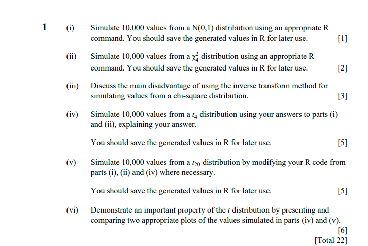
Simulate 10,000 values from a N(0,1) distribution using an appropriate R command. You should save the generated values in R for later use. [1]

remember we use rnorm(n,mean,std) , in our case mean is 0 and 1 is std

Question (ii)

Simulate 10,000 values from a $\chi^2_4$ distribution using an appropriate R command. You should save the generated values in R for later use. [2]

like in normal distributionrchisq(n,df), in our case df is4`

Question (iv)

Simulate 10,000 values from a t4 distribution using your answers to parts (i) and (ii), explaining your answer. You should save the generated values in R for later use. [5]

when given the $\chi^2$ distribution and standard normal distribution we can make use of the transformation that says .

\[t_{n} = \frac{Z}{\sqrt{\frac{\chi^2_n}{n}}}\]

Question (v)

Simulate 10,000 values from a t20 distribution by modifying your R code from parts (i), (ii) and (iv) where necessary. You should save the generated values in R for later use. [5]

when given the $\chi^2$ distribution and standard normal distribution we can make use of the transformation that says .

\[t_{n} = \frac{Z}{\sqrt{\frac{\chi^2_n}{n}}}\]

Probability Distributions to ACE your CS1 EXAM

Mathematical Representations of Distributions

Probability distributions in R

Discrete Random Variables

Binary Random Variable

Binomial Random Variable

Continuous Random Variables

Exponential Random Variable

Gamma Random Variable

Normal (Gaussian) Random Variable

Beta Random Variable

Distributions Used in Testing

\(\chi^2\) Distribution

Student’s \(t\)-Distribution

\(F\)-Distribution

Subject CS1 – Actuarial Practice Core Principles

Question (ii)

Question (iv)

Question (v)