sales<-tribble(~ year , ~country , ~product    , ~profit ,~Own ,~Time,
                 2000 , "Finland", "Computer"  ,   1500  ,"Y"  ,"D",
                 2000 , "Finland" ,"Phone"      ,   100   ,"Y"  ,"D",
                 2001 , "Finland" ,"Phone"      ,     10  ,"N"  ,"D",
                 2000 , "India"   ,"Calculator" ,     75  ,"Y"  ,"E",
                 2000 , "India"   ,"Calculator" ,     75  ,"N"  ,"E",
                 2000 , "India"   ,"Computer"   ,   1200  ,"N"  ,"E",
                 2000 , "USA"     , "Calculator",     75  ,"Y"  ,"E",
                 2000 , "USA"     , "Computer"  ,   1500  ,"N"  ,"E",
                 2001 , "USA"     ,"Calculator" ,     50  ,"Y"  ,"E",
                 2001 , "USA"     ,"Computer"   ,   1500  ,"Y"  ,"E",
                 2001 , "USA"     ,"Computer"   ,   1200  ,"Y"  ,"D",
                 2001 , "USA"     , "TV"        ,    150  ,"Y"  ,"D",
                 2001 , "USA"     , "TV"        ,    100  ,"Y"  ,"D")
sales
#> # A tibble: 13 × 6
#>     year country product    profit Own   Time
#>    <dbl> <chr>   <chr>       <dbl> <chr> <chr>
#>  1  2000 Finland Computer     1500 Y     D
#>  2  2000 Finland Phone         100 Y     D
#>  3  2001 Finland Phone          10 N     D
#>  4  2000 India   Calculator     75 Y     E
#>  5  2000 India   Calculator     75 N     E
#>  6  2000 India   Computer     1200 N     E
#>  7  2000 USA     Calculator     75 Y     E
#>  8  2000 USA     Computer     1500 N     E
#>  9  2001 USA     Calculator     50 Y     E
#> 10  2001 USA     Computer     1500 Y     E
#> 11  2001 USA     Computer     1200 Y     D
#> 12  2001 USA     TV            150 Y     D
#> 13 2001 USA TV 100 Y DSQL and R compared
databases
sql training
data manipulation
Comparing R and SQL
Loading data
The Notebook is divided into tabbed sections as seen below.
loading data in R
loading data in SQL
CREATE TABLE profits (sales_id INT PRIMARY KEY,
                     year INT,
                     country VARCHAR(50),
                     product VARCHAR(50),
                     profit DECIMAL(10,2)
                     );

INSERT INTO profits VALUES (1,2000 , "Finland", "Computer"  ,   1500 ),
                 (2,2000 , "Finland" ,"Phone"      ,   100 ),
                 (3,2001 , "Finland" ,"Phone"      ,     10),
                 (4,2000 , "India"   ,"Calculator" ,     75),
                 (5,2000 , "India"   ,"Calculator" ,     75),
                 (6,2000 , "India"   ,"Computer"   ,   1200),
                 (7,2000 , "USA"     , "Calculator",     75),
                 (8,2000 , "USA"     , "Computer"  ,   1500),
                 (9,2001 , "USA"     ,"Calculator" ,     50),
                 (10,2001 , "USA"     ,"Computer"   ,   1500),
                 (11,2001 , "USA"     ,"Computer"   ,   1200),
                 (12,2001 , "USA"     , "TV"        ,    150),
                 (13,2001 , "USA"     , "TV"        ,    100);
#> # A tibble: 13 × 6
#>     year country product    profit Own   Time
#>    <dbl> <chr>   <chr>       <dbl> <chr> <chr>
#>  1  2000 Finland Computer     1500 Y     D
#>  2  2000 Finland Phone         100 Y     D
#>  3  2001 Finland Phone          10 N     D
#>  4  2000 India   Calculator     75 Y     E
#>  5  2000 India   Calculator     75 N     E
#>  6  2000 India   Computer     1200 N     E
#>  7  2000 USA     Calculator     75 Y     E
#>  8  2000 USA     Computer     1500 N     E
#>  9  2001 USA     Calculator     50 Y     E
#> 10  2001 USA     Computer     1500 Y     E
#> 11  2001 USA     Computer     1200 Y     D
#> 12  2001 USA     TV            150 Y     D
#> 13  2001 USA     TV            100 Y     D
Selecting columns
selecting columns in R
sales |> select(everything())
#> # A tibble: 13 × 6
#>     year country product    profit Own   Time
#>    <dbl> <chr>   <chr>       <dbl> <chr> <chr>
#>  1  2000 Finland Computer     1500 Y     D
#>  2  2000 Finland Phone         100 Y     D
#>  3  2001 Finland Phone          10 N     D
#>  4  2000 India   Calculator     75 Y     E
#>  5  2000 India   Calculator     75 N     E
#>  6  2000 India   Computer     1200 N     E
#>  7  2000 USA     Calculator     75 Y     E
#>  8  2000 USA     Computer     1500 N     E
#>  9  2001 USA     Calculator     50 Y     E
#> 10  2001 USA     Computer     1500 Y     E
#> 11  2001 USA     Computer     1200 Y     D
#> 12  2001 USA     TV            150 Y     D
#> 13  2001 USA     TV            100 Y     D
selecting all columns in SQL
SELECT *
FROM sales;| year | country | product | profit | Own | Time |
|---|---|---|---|---|---|
| 2000 | Finland | Computer | 1500 | Y | D |
| 2000 | Finland | Phone | 100 | Y | D |
| 2001 | Finland | Phone | 10 | N | D |
| 2000 | India | Calculator | 75 | Y | E |
| 2000 | India | Calculator | 75 | N | E |
| 2000 | India | Computer | 1200 | N | E |
| 2000 | USA | Calculator | 75 | Y | E |
| 2000 | USA | Computer | 1500 | N | E |
| 2001 | USA | Calculator | 50 | Y | E |
| 2001 | USA | Computer | 1500 | Y | E |
Select a subset of columns
selecting subset columns in R
sales |>
  select(year,country,product)
#> # A tibble: 13 × 3
#>     year country product
#>    <dbl> <chr>   <chr>
#>  1  2000 Finland Computer
#>  2  2000 Finland Phone
#>  3  2001 Finland Phone
#>  4  2000 India   Calculator
#>  5  2000 India   Calculator
#>  6  2000 India   Computer
#>  7  2000 USA     Calculator
#>  8  2000 USA     Computer
#>  9  2001 USA     Calculator
#> 10  2001 USA     Computer
#> 11  2001 USA     Computer
#> 12  2001 USA     TV
#> 13  2001 USA     TV
selecting subset columns in SQL
SELECT year,country,product
FROM sales;| year | country | product |
|---|---|---|
| 2000 | Finland | Computer |
| 2000 | Finland | Phone |
| 2001 | Finland | Phone |
| 2000 | India | Calculator |
| 2000 | India | Calculator |
| 2000 | India | Computer |
| 2000 | USA | Calculator |
| 2000 | USA | Computer |
| 2001 | USA | Calculator |
| 2001 | USA | Computer |
filtering data
Filtering data in R
sales |>
  filter(product=="Computer")
#> # A tibble: 5 × 6
#>    year country product  profit Own   Time
#>   <dbl> <chr>   <chr>     <dbl> <chr> <chr>
#> 1  2000 Finland Computer   1500 Y     D
#> 2  2000 India   Computer   1200 N     E
#> 3  2000 USA     Computer   1500 N     E
#> 4  2001 USA     Computer   1500 Y     E
#> 5  2001 USA     Computer   1200 Y     D
Filtering data in SQL
SELECT *
FROM sales
WHERE product='Computer';| year | country | product | profit | Own | Time |
|---|---|---|---|---|---|
| 2000 | Finland | Computer | 1500 | Y | D |
| 2000 | India | Computer | 1200 | N | E |
| 2000 | USA | Computer | 1500 | N | E |
| 2001 | USA | Computer | 1500 | Y | E |
| 2001 | USA | Computer | 1200 | Y | D |
filtering with AND
Filtering data in R
sales |>
  filter(product=="Computer" & year=="2001")
#> # A tibble: 2 × 6
#>    year country product  profit Own   Time
#>   <dbl> <chr>   <chr>     <dbl> <chr> <chr>
#> 1  2001 USA     Computer   1500 Y     E
#> 2  2001 USA     Computer   1200 Y     D
Filtering data in SQL
SELECT *
FROM sales
WHERE product='Computer' AND year='2001';| year | country | product | profit | Own | Time |
|---|---|---|---|---|---|
| 2001 | USA | Computer | 1500 | Y | E |
| 2001 | USA | Computer | 1200 | Y | D |
filtering with OR
Filtering data in R
sales |>
  filter(product=="Computer"| country=="USA")
#> # A tibble: 9 × 6
#>    year country product    profit Own   Time
#>   <dbl> <chr>   <chr>       <dbl> <chr> <chr>
#> 1  2000 Finland Computer     1500 Y     D
#> 2  2000 India   Computer     1200 N     E
#> 3  2000 USA     Calculator     75 Y     E
#> 4  2000 USA     Computer     1500 N     E
#> 5  2001 USA     Calculator     50 Y     E
#> 6  2001 USA     Computer     1500 Y     E
#> 7  2001 USA     Computer     1200 Y     D
#> 8  2001 USA     TV            150 Y     D
#> 9  2001 USA     TV            100 Y     D
Filtering data in SQL
SELECT *
FROM sales
WHERE product='Computer' OR country='USA';| year | country | product | profit | Own | Time |
|---|---|---|---|---|---|
| 2000 | Finland | Computer | 1500 | Y | D |
| 2000 | India | Computer | 1200 | N | E |
| 2000 | USA | Calculator | 75 | Y | E |
| 2000 | USA | Computer | 1500 | N | E |
| 2001 | USA | Calculator | 50 | Y | E |
| 2001 | USA | Computer | 1500 | Y | E |
| 2001 | USA | Computer | 1200 | Y | D |
| 2001 | USA | TV | 150 | Y | D |
| 2001 | USA | TV | 100 | Y | D |
filtering with BETWEEN
Filtering data in R
sales |>
  filter(between(profit,0,100))
#> # A tibble: 7 × 6
#>    year country product    profit Own   Time
#>   <dbl> <chr>   <chr>       <dbl> <chr> <chr>
#> 1  2000 Finland Phone         100 Y     D
#> 2  2001 Finland Phone          10 N     D
#> 3  2000 India   Calculator     75 Y     E
#> 4  2000 India   Calculator     75 N     E
#> 5  2000 USA     Calculator     75 Y     E
#> 6  2001 USA     Calculator     50 Y     E
#> 7  2001 USA     TV            100 Y     D
Filtering data in SQL
SELECT *
FROM sales
WHERE profit BETWEEN 0 AND 100;| year | country | product | profit | Own | Time |
|---|---|---|---|---|---|
| 2000 | Finland | Phone | 100 | Y | D |
| 2001 | Finland | Phone | 10 | N | D |
| 2000 | India | Calculator | 75 | Y | E |
| 2000 | India | Calculator | 75 | N | E |
| 2000 | USA | Calculator | 75 | Y | E |
| 2001 | USA | Calculator | 50 | Y | E |
| 2001 | USA | TV | 100 | Y | D |
Arranging data
Arranging data in R
sales |>
  arrange(profit)
#> # A tibble: 13 × 6
#>     year country product    profit Own   Time
#>    <dbl> <chr>   <chr>       <dbl> <chr> <chr>
#>  1  2001 Finland Phone          10 N     D
#>  2  2001 USA     Calculator     50 Y     E
#>  3  2000 India   Calculator     75 Y     E
#>  4  2000 India   Calculator     75 N     E
#>  5  2000 USA     Calculator     75 Y     E
#>  6  2000 Finland Phone         100 Y     D
#>  7  2001 USA     TV            100 Y     D
#>  8  2001 USA     TV            150 Y     D
#>  9  2000 India   Computer     1200 N     E
#> 10  2001 USA     Computer     1200 Y     D
#> 11  2000 Finland Computer     1500 Y     D
#> 12  2000 USA     Computer     1500 N     E
#> 13  2001 USA     Computer     1500 Y     E
Arranging data in SQL
SELECT *
FROM sales
ORDER BY profit;| year | country | product | profit | Own | Time |
|---|---|---|---|---|---|
| 2001 | Finland | Phone | 10 | N | D |
| 2001 | USA | Calculator | 50 | Y | E |
| 2000 | India | Calculator | 75 | Y | E |
| 2000 | India | Calculator | 75 | N | E |
| 2000 | USA | Calculator | 75 | Y | E |
| 2000 | Finland | Phone | 100 | Y | D |
| 2001 | USA | TV | 100 | Y | D |
| 2001 | USA | TV | 150 | Y | D |
| 2000 | India | Computer | 1200 | N | E |
| 2001 | USA | Computer | 1200 | Y | D |
Arranging data in DESC order
arranging data in R
sales |>
  arrange(desc(profit))
#> # A tibble: 13 × 6
#>     year country product    profit Own   Time
#>    <dbl> <chr>   <chr>       <dbl> <chr> <chr>
#>  1  2000 Finland Computer     1500 Y     D
#>  2  2000 USA     Computer     1500 N     E
#>  3  2001 USA     Computer     1500 Y     E
#>  4  2000 India   Computer     1200 N     E
#>  5  2001 USA     Computer     1200 Y     D
#>  6  2001 USA     TV            150 Y     D
#>  7  2000 Finland Phone         100 Y     D
#>  8  2001 USA     TV            100 Y     D
#>  9  2000 India   Calculator     75 Y     E
#> 10  2000 India   Calculator     75 N     E
#> 11  2000 USA     Calculator     75 Y     E
#> 12  2001 USA     Calculator     50 Y     E
#> 13  2001 Finland Phone          10 N     D
arranging data in SQL
SELECT *
FROM sales
ORDER BY profit DESC;| year | country | product | profit | Own | Time |
|---|---|---|---|---|---|
| 2000 | Finland | Computer | 1500 | Y | D |
| 2000 | USA | Computer | 1500 | N | E |
| 2001 | USA | Computer | 1500 | Y | E |
| 2000 | India | Computer | 1200 | N | E |
| 2001 | USA | Computer | 1200 | Y | D |
| 2001 | USA | TV | 150 | Y | D |
| 2000 | Finland | Phone | 100 | Y | D |
| 2001 | USA | TV | 100 | Y | D |
| 2000 | India | Calculator | 75 | Y | E |
| 2000 | India | Calculator | 75 | N | E |
Mutating new columns
Mutating new columns in R
sales |>
  mutate(profit=profit/1000)
#> # A tibble: 13 × 6
#>     year country product    profit Own   Time
#>    <dbl> <chr>   <chr>       <dbl> <chr> <chr>
#>  1  2000 Finland Computer    1.5   Y     D
#>  2  2000 Finland Phone       0.1   Y     D
#>  3  2001 Finland Phone       0.01  N     D
#>  4  2000 India   Calculator  0.075 Y     E
#>  5  2000 India   Calculator  0.075 N     E
#>  6  2000 India   Computer    1.2   N     E
#>  7  2000 USA     Calculator  0.075 Y     E
#>  8  2000 USA     Computer    1.5   N     E
#>  9  2001 USA     Calculator  0.05  Y     E
#> 10  2001 USA     Computer    1.5   Y     E
#> 11  2001 USA     Computer    1.2   Y     D
#> 12  2001 USA     TV          0.15  Y     D
#> 13  2001 USA     TV          0.1   Y     D
Mutating new columns in SQL
SELECT profit/1000 AS profit,*
FROM sales;| profit | year | country | product | profit | Own | Time |
|---|---|---|---|---|---|---|
| 1.500 | 2000 | Finland | Computer | 1500 | Y | D |
| 0.100 | 2000 | Finland | Phone | 100 | Y | D |
| 0.010 | 2001 | Finland | Phone | 10 | N | D |
| 0.075 | 2000 | India | Calculator | 75 | Y | E |
| 0.075 | 2000 | India | Calculator | 75 | N | E |
| 1.200 | 2000 | India | Computer | 1200 | N | E |
| 0.075 | 2000 | USA | Calculator | 75 | Y | E |
| 1.500 | 2000 | USA | Computer | 1500 | N | E |
| 0.050 | 2001 | USA | Calculator | 50 | Y | E |
| 1.500 | 2001 | USA | Computer | 1500 | Y | E |
Summarizing data
Summarizing data in R
sales |>
  summarize(mean_profit=mean(profit),
            count = n())
#> # A tibble: 1 × 2
#>   mean_profit count
#>         <dbl> <int>
#> 1        580.    13
Summarizing data in SQL
SELECT AVG(profit) AS mean_profit,
       COUNT(*) AS count
FROM sales;| mean_profit | count |
|---|---|
| 579.6154 | 13 |
Grouping and Summarizing data
Grouping and Summarizing data in R
sales |>
  group_by(year) |>
  summarize(mean_profit=mean(profit),
            count = n())
#> # A tibble: 2 × 3
#>    year mean_profit count
#>   <dbl>       <dbl> <int>
#> 1  2000        646.     7
#> 2  2001        502.     6
Grouping and Summarizing data in SQL
SELECT year,
       AVG(profit) AS mean_profit,
       COUNT(*) AS count
FROM sales
GROUP BY year;| year | mean_profit | count |
|---|---|---|
| 2000 | 646.4286 | 7 |
| 2001 | 501.6667 | 6 |
data for joins
generally the following step show how a join is done in SQL
-
SELECTt1.comon_column1,t1.common_column2,… -
FROMtable1ASt1 -
<type> JOINtable2ASt2 -
ONt1.common_unique_column = t2.common_unique_column;
data for joins in R
join_df1
#>        A B C
#> 1    red 2 3
#> 2 orange 4 6
#> 3 yellow 8 9
#> 4  green 0 0
#> 5 indigo 3 3
#> 6   blue 1 1
#> 7 purple 5 5
#> 8  white 8 2
join_df2
#> A D
#> 1 red 3
#> 2 orange 5
#> 3 yellow 7
#> 4 green 1
#> 5 indigo 3
#> 6 blue 6
#> 7 pink 9data for joins in SQL
SELECT *
FROM join_df1;| A | B | C |
|---|---|---|
| red | 2 | 3 |
| orange | 4 | 6 |
| yellow | 8 | 9 |
| green | 0 | 0 |
| indigo | 3 | 3 |
| blue | 1 | 1 |
| purple | 5 | 5 |
| white | 8 | 2 |
SELECT *
FROM join_df2;| A | D |
|---|---|
| red | 3 |
| orange | 5 |
| yellow | 7 |
| green | 1 |
| indigo | 3 |
| blue | 6 |
| pink | 9 |
inner join
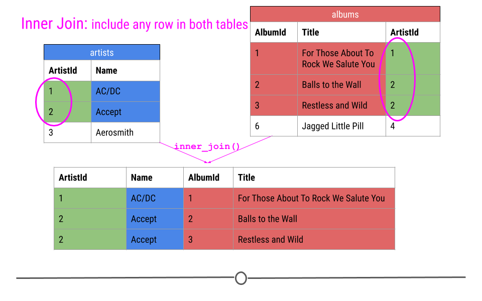
inner join in R
join_df1 |>
  inner_join(join_df2, by = "A")
#>        A B C D
#> 1    red 2 3 3
#> 2 orange 4 6 5
#> 3 yellow 8 9 7
#> 4  green 0 0 1
#> 5 indigo 3 3 3
#> 6   blue 1 1 6
inner join in SQL
SELECT *
FROM join_df1 AS j1
INNER JOIN join_df2 AS j2
ON j1.A=j2.A;| A | B | C | A | D |
|---|---|---|---|---|
| red | 2 | 3 | red | 3 |
| orange | 4 | 6 | orange | 5 |
| yellow | 8 | 9 | yellow | 7 |
| green | 0 | 0 | green | 1 |
| indigo | 3 | 3 | indigo | 3 |
| blue | 1 | 1 | blue | 6 |
left join
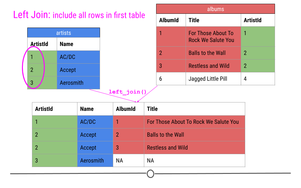
left join in R
join_df1 |>
left_join(join_df2, by = "A")
#>        A B C  D
#> 1    red 2 3  3
#> 2 orange 4 6  5
#> 3 yellow 8 9  7
#> 4  green 0 0  1
#> 5 indigo 3 3  3
#> 6   blue 1 1  6
#> 7 purple 5 5 NA
#> 8  white 8 2 NA
left join in SQL
SELECT j1.A,B,C,D
FROM join_df1 AS j1
LEFT JOIN join_df2 AS j2
ON j1.A=j2.A| A | B | C | D |
|---|---|---|---|
| red | 2 | 3 | 3 |
| orange | 4 | 6 | 5 |
| yellow | 8 | 9 | 7 |
| green | 0 | 0 | 1 |
| indigo | 3 | 3 | 3 |
| blue | 1 | 1 | 6 |
| purple | 5 | 5 | NA |
| white | 8 | 2 | NA |
Right join
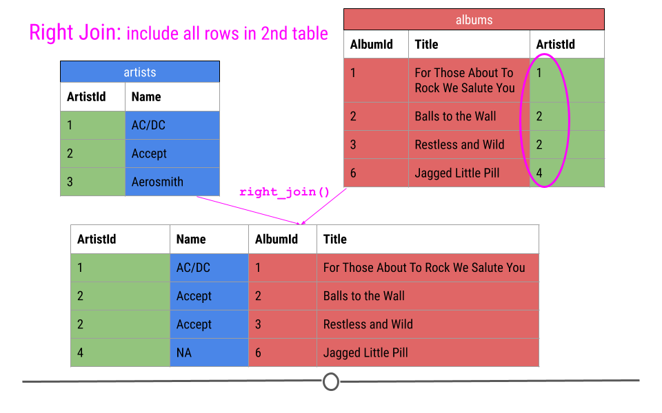
Right join in R
join_df1 |>
right_join(join_df2, by = "A")
#>        A  B  C D
#> 1    red  2  3 3
#> 2 orange  4  6 5
#> 3 yellow  8  9 7
#> 4  green  0  0 1
#> 5 indigo  3  3 3
#> 6   blue  1  1 6
#> 7   pink NA NA 9
Right join in SQL
SELECT j2.A,B,C,D
FROM join_df1 AS j1
RIGHT JOIN join_df2 AS j2
ON j1.A=j2.A| A | B | C | D |
|---|---|---|---|
| red | 2 | 3 | 3 |
| orange | 4 | 6 | 5 |
| yellow | 8 | 9 | 7 |
| green | 0 | 0 | 1 |
| indigo | 3 | 3 | 3 |
| blue | 1 | 1 | 6 |
| pink | NA | NA | 9 |
Full join
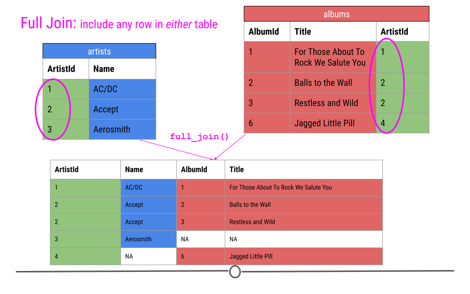
full join in R
join_df1 |>
full_join(join_df2, by = "A")
#>        A  B  C  D
#> 1    red  2  3  3
#> 2 orange  4  6  5
#> 3 yellow  8  9  7
#> 4  green  0  0  1
#> 5 indigo  3  3  3
#> 6   blue  1  1  6
#> 7 purple  5  5 NA
#> 8  white  8  2 NA
#> 9   pink NA NA  9
full join in SQL
SELECT j1.A,B,C,D
FROM join_df1 AS j1
FULL JOIN join_df2 AS j2
ON j1.A=j2.A| A | B | C | D |
|---|---|---|---|
| red | 2 | 3 | 3 |
| orange | 4 | 6 | 5 |
| yellow | 8 | 9 | 7 |
| green | 0 | 0 | 1 |
| indigo | 3 | 3 | 3 |
| blue | 1 | 1 | 6 |
| purple | 5 | 5 | NA |
| white | 8 | 2 | NA |
| NA | NA | NA | 9 |