Machine Learning Approaches for Auto Insurance

School of Mathematics and Statistics

The growing trend in the number and severity of auto insurance claims creates a need for new methods to efficiently handle these claims. Machine learning (ML) is one of the methods that solves this problem. As car insurers aim to improve their customer service, these companies have started adopting and applying ML to enhance the interpretation and comprehension of their data for efficiency, thus improving their customer service through a better understanding of their needs. This study considers how automotive insurance providers incorporate machinery learning in their company, and explores how ML models can apply to insurance big data. We utilize various ML methods, such as logistic regression and K-NN, to predict claim occurrence. Furthermore, we evaluate and compare these models’ performances.

Author

Bongani Ncube

Published

14 March 2024

Description: In this qmd, I evaluate different supervised machine learning algorithms for predicting Autoinsurance.

Introduction

I once carried out a study using this data on B Ncube Analysis

Methods

To get started, there are several packages I will be using. Tidyverse packages help with further cleaning and preparing data. Tidymodels packages have almost all of what I need for the machine learning steps. kknn helps me build my knn model. knitr is used to create kable tables. baguette is used in my bagging model. doParallel allows for parallel computing on my laptop. vip helps to identify variable importance.

Data Preprocessing

First I read in the data. These data were cleaned and joined in a separate script, but they will still need a bit of preprocessing. The outcome variable in this dataset is labeled target_flag and indicates if at risk (1) or not (0). I start out by exploring the data dimensions.

VARIABLE NAME	DEFINITION	THEORETICAL EFFECT
INDEX	Identification Variable (do not use)	None
TARGET_FLAG	Was Car in a crash? 1=YES 0=NO	None
TARGET_AMT	If car was in a crash, what was the cost	None
AGE	Age of Driver	Very young people tend to be risky. Maybe very old people also.
BLUEBOOK	Value of Vehicle	Unknown effect on probability of collision, but probably effect the payout if there is a crash
CAR_AGE	Vehicle Age	Unknown effect on probability of collision, but probably effect the payout if there is a crash
CAR_TYPE	Type of Car	Unknown effect on probability of collision, but probably effect the payout if there is a crash
CAR_USE	Vehicle Use	Commercial vehicles are driven more, so might increase probability of collision
CLM_FREQ	#Claims(Past 5 Years)	The more claims you filed in the past, the more you are likely to file in the future
EDUCATION	Max Education Level	Unknown effect, but in theory more educated people tend to drive more safely
HOMEKIDS	#Children @Home	Unknown effect
HOME_VAL	Home Value	In theory, home owners tend to drive more responsibly
INCOME	Income	In theory, rich people tend to get into fewer crashes
JOB	Job Category	In theory, white collar jobs tend to be safer
KIDSDRIV	#Driving Children	When teenagers drive your car, you are more likely to get into crashes
MSTATUS	Marital Status	In theory, married people drive more safely
MVR_PTS	Motor Vehicle Record Points	If you get lots of traffic tickets, you tend to get into more crashes
OLDCLAIM	Total Claims(Past 5 Years)	If your total payout over the past five years was high, this suggests future payouts will be high
PARENT1	Single Parent	Unknown effect
RED_CAR	A Red Car	Urban legend says that red cars (especially red sports cars) are more risky. Is that true?
REVOKED	License Revoked (Past 7 Years)	If your license was revoked in the past 7 years, you probably are a more risky driver.
SEX	Gender	Urban legend says that women have less crashes then men. Is that true?
TIF	Time in Force	People who have been customers for a long time are usually more safe.
TRAVTIME	Distance to Work	Long drives to work usually suggest greater risk
URBANICITY	Home/Work Area	Unknown
YOJ	Years on Job	People who stay at a job for a long time are usually more safe

Explore some characteristics of the dataset

	Count
Number of Columns	25
Number of Rows	8161

Target Flag	Count	proportion
0	0.7361843	74%
1	0.2638157	26%

Data Prep

There are a lot on NA values in this dataset. I have a lot of columns already, so I can reduce that by removing columns that have a high proportion of NA values. Here I only keep columns where less than 20% of rows have NA values.

# Calculate the proportion of NA values in each column
na_proportion <- colMeans(is.na(out_new), na.rm = TRUE)

#I want to remove rows with extreme NA counts (more than 20%)
# Define the threshold (20% or 0.20)
threshold <- 0.20

# Find columns with more than the threshold proportion of NA values
columns_meeting_threshold <- names(na_proportion[na_proportion <= threshold])

# Print the column names that meet the threshold
columns_meeting_threshold %>% kable(col.names = "Columns that are below NA threshold")

Columns that are below NA threshold
target_flag
target_amt
kidsdriv
age
homekids
yoj
income
parent1
home_val
mstatus
sex
education
job
travtime
car_use
bluebook
tif
car_type
red_car
oldclaim
clm_freq
revoked
mvr_pts
car_age
urbanicity


# Select for just those columns that meet my criteria
fish_short <- out_new %>% 
  select(all_of(columns_meeting_threshold))

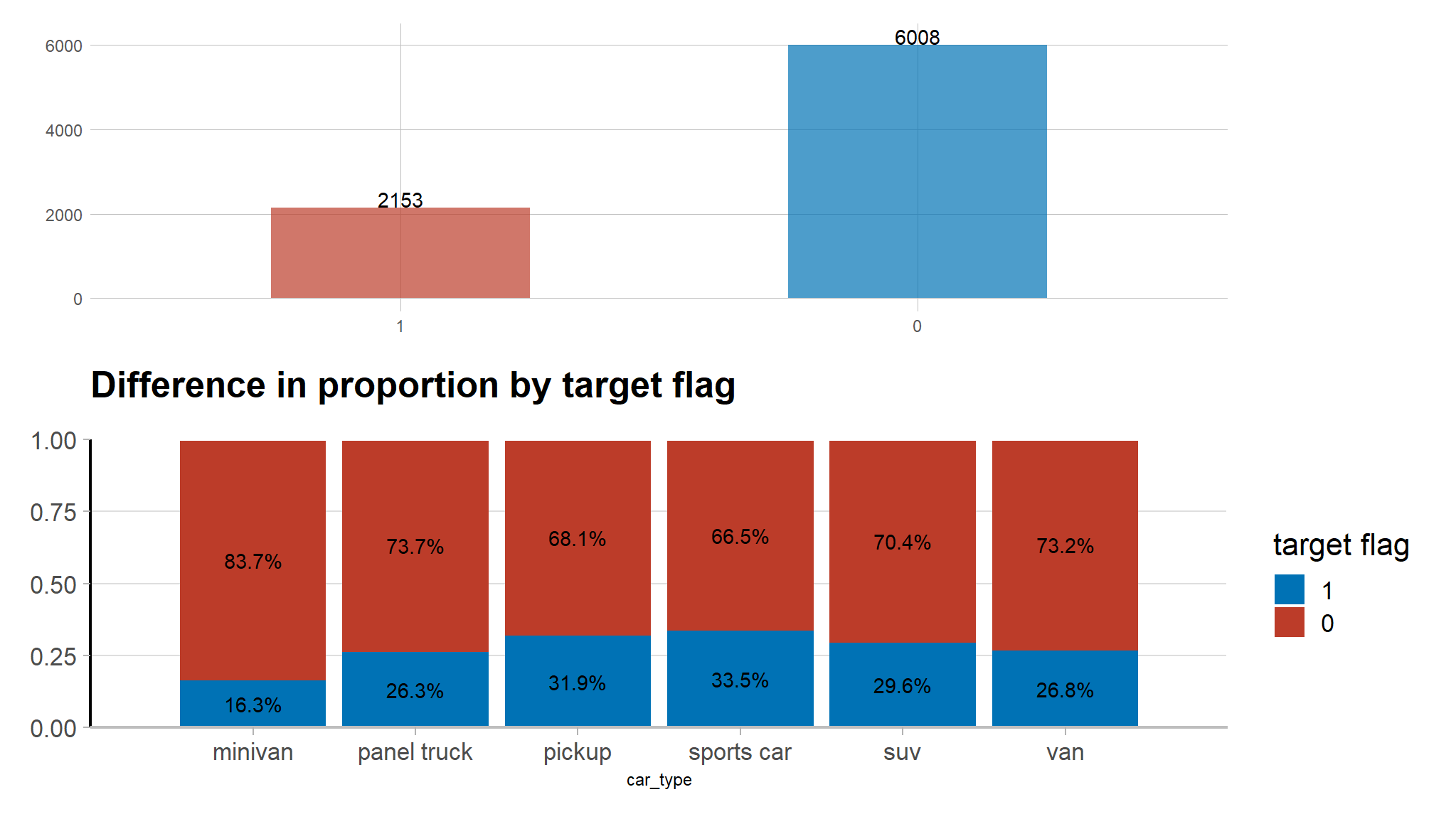
Note

The figure shows that the target variable is heavily imbalanced, with class 0 having 74% observations and class 1 having only 24% observations

Data Budgetting

# Stratified split 
auto_split<-out_new |> 
  mutate(target_flag=as.factor(target_flag))|> 
  initial_split(strata = target_flag, prop = 0.7)

# Obtain train and test sets
train <- training(auto_split)
test <- testing(auto_split)

# Print out observations in each category
glue::glue(
  'The training set has {nrow(train)} observations \n',
  'The testing set has {nrow(test)} observations'
)
#> The training set has 5712 observations 
#> The testing set has 2449 observations

Preprocessing

I create a recipe for the preprocessing steps used. I use dummy columns to make all the factor (categorical) variables have their own column. I remove columns where there is no variation in the data. Then I normalize the numeric columns because the lasso and knn algorithms require normalization to avoid certain features dominating the model. I use the same preprocessing steps for all algorithms for adequate comparison.

# Data preprocessing with recipes
boost_recipe <- recipe(target_flag ~., data=train) |>
  step_select(!target_amt) |>
  step_impute_bag(all_numeric_predictors())|>#impute numerical data
  step_impute_mode(all_nominal_predictors())|>#impute nominal data
  step_YeoJohnson(all_numeric_predictors())|># approximate near normal distributions (optional here)
  step_normalize(all_numeric_predictors())|># center and scale numerical vars 
  step_dummy(all_nominal_predictors(), -all_outcomes(), one_hot = TRUE)|># keep ref levels with one hot
  step_nzv(all_numeric_predictors())|># remove numeric vars that have zero variance (single unique value)
  step_corr(all_predictors(), threshold = 0.5, method = 'spearman')|># address collinearity
  themis::step_smote(target_flag) # rebalance the dataset based on the response variable

# Check test and train dfs look as expected
prepped <- boost_recipe %>% 
  prep()
claim_baked_train <- bake(prepped,train)
claim_baked_test <- bake(prepped, test)

Dummy Classifier

Because my data are unbalanced , if a model always chose 0 it would have a high accuracy. Of course, that is not very helpful when trying to predict . Here I derive a dummy accuracy by calculating the accuracy of a model that always predicts non-threatened. This will serve as a baseline for if a model is performing well (better than the dummy) or not.

# Calculate dummy classifier for baseline comparison
# Calculate the number of rows where target_flag is 0
num_is_0 <- sum(test$target_flag == 0)

# Calculate the number of rows where target_flag is not 0
num_is_not_0 <- nrow(test) - num_is_0

# Calculate the accuracy of the dummy classifier (always predicting the majority class)
dummy <- num_is_0 / nrow(test)

The dummy classifier accuracy is 0.736. This will serve as the baseline for other algorithms. Now I will proceed with building various models and training with the training data. I will be building Lasso and K-Nearest Neighbors.

10 Fold cross validation

set.seed(123)

# Set up k-fold cross validation with 10 folds. This can be used for all the algorithms
fish_cv = train %>% 
  vfold_cv(v = 10,
           strata = target_flag)

Lasso for Classification on validation set

# Set specifications
tune_l_spec <- logistic_reg(penalty = tune(), 
                            mixture = 1) %>%
               set_engine("glmnet")

# Define a workflow
wf_l <- workflow() %>%
  add_model(tune_l_spec) %>% 
  add_recipe(boost_recipe)
# set grid
lambda_grid <- grid_regular(penalty(), levels = 50)

doParallel::registerDoParallel()
set.seed(123)

# Tune lasso model
lasso_grid <-   wf_l %>% 
  tune_grid(
    add_model(tune_l_spec),
    resamples = fish_cv,
    grid = lambda_grid
)

# Plot the mean accuracy and AUC at each penalty
lasso_grid %>%
  collect_metrics() %>%
  ggplot(aes(penalty, mean, color = .metric)) +
  geom_errorbar(aes(ymin = mean - std_err,
                    ymax = mean + std_err),
                alpha = 0.5) +
  geom_line(size = 1.5) +
  facet_wrap(~.metric, 
             scales = "free", 
             strip.position = "left",
             nrow = 2, labeller = as_labeller(c(`accuracy` = "Accuracy", 
                                                `roc_auc` = "Area under ROC curve"))) +
  scale_x_log10(name = "Penalty") +
  scale_y_continuous(name = "") +
  scale_color_manual(values = c("#4a6c75", "#57ba72")) +
  theme_minimal() +
  theme(
    strip.placement = "outside",
    legend.position = "none",
    panel.background = element_blank(),
    plot.background = element_blank()
  ) +
  labs(title = "Results of penalty tuning")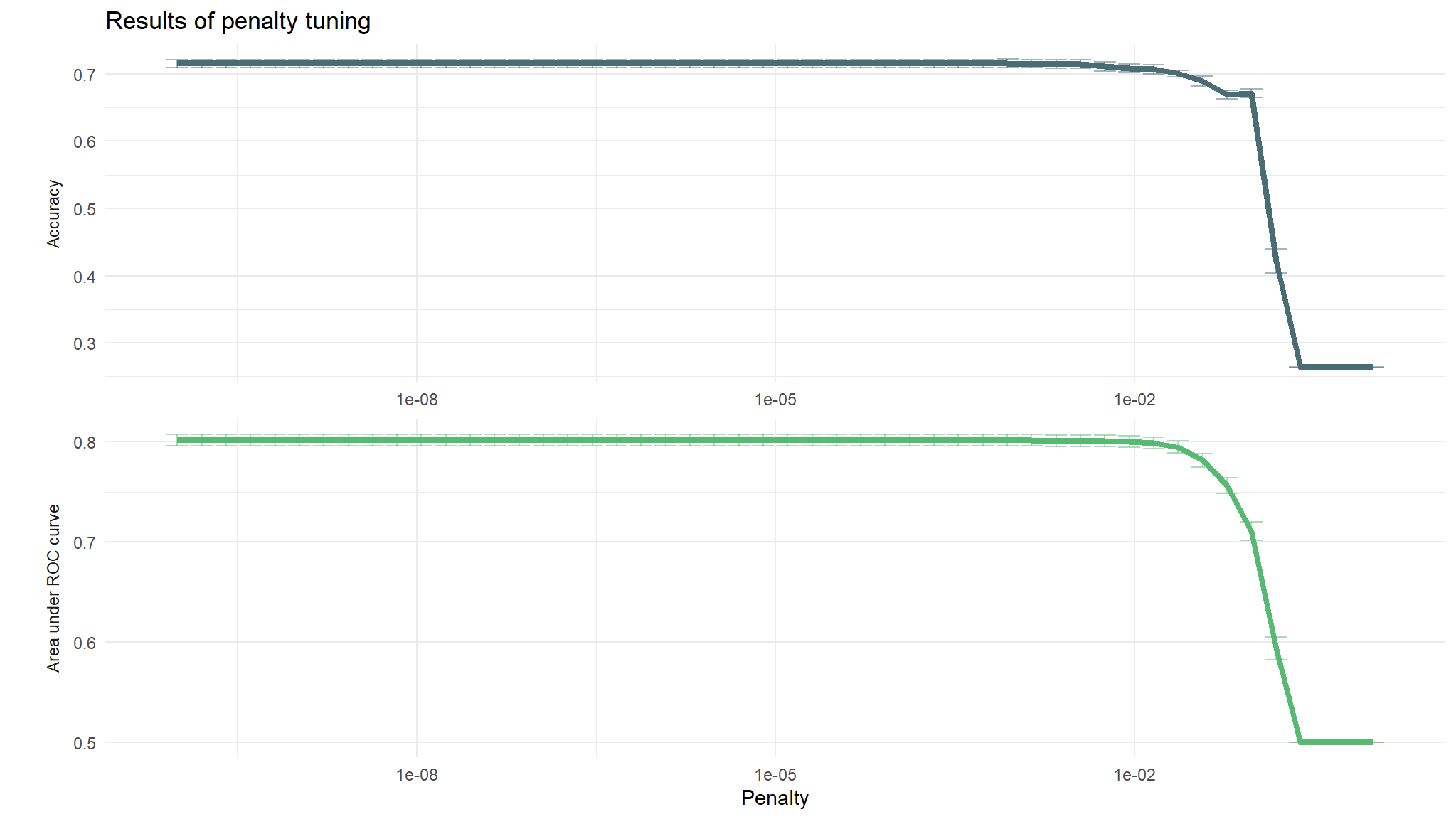


# View table
lasso_grid %>%
  tune::show_best(metric = "roc_auc") %>%
  slice_head(n = 5) %>% 
  kable(caption = "Performance of the best models and the associated estimates for the penalty parameter values.")

Performance of the best models and the associated estimates for the penalty parameter values.
penalty	.metric	.estimator	mean	n	std_err	.config
0.0008685	roc_auc	binary	0.8017635	10	0.0057321	Preprocessor1_Model35
0.0005429	roc_auc	binary	0.8017161	10	0.0057545	Preprocessor1_Model34
0.0003393	roc_auc	binary	0.8016640	10	0.0057542	Preprocessor1_Model33
0.0002121	roc_auc	binary	0.8015609	10	0.0057884	Preprocessor1_Model32
0.0000000	roc_auc	binary	0.8015371	10	0.0057962	Preprocessor1_Model01


# Select the model with the highest auc
best_lasso <- lasso_grid %>%
  select_best("roc_auc")

final_l_wf <- wf_l %>% 
  finalize_workflow(best_lasso)

# Perform a last fit to see how the model performs on the test data
final_lasso_fit <- last_fit(final_l_wf, auto_split)

# Collect metrics on the test data
tibble_lasso <- final_lasso_fit %>% collect_metrics()
tibble_lasso %>% 
  kable(caption = "Accuracy and area under ther receiver operator curve of the final fit.")

Accuracy and area under ther receiver operator curve of the final fit.
.metric	.estimator	.estimate	.config
accuracy	binary	0.7113107	Preprocessor1_Model1
roc_auc	binary	0.7904190	Preprocessor1_Model1


# Grab the model accuracy on the testing data
final_lasso_accuracy <- tibble_lasso %>%
  filter(.metric == "accuracy") %>%
  pull(.estimate)
final_lasso_auc <- tibble_lasso %>%
  filter(.metric == "roc_auc") %>%
  pull(.estimate)

# Bind predictions and original data
lasso_test_rs <- cbind(test, final_lasso_fit$.predictions)[, -16]# Remove duplicate column

# Compute a confusion matrix
cm_lasso <- lasso_test_rs %>% yardstick::conf_mat(truth = target_flag, estimate = .pred_class) 

# Create a custom color palette
custom_palette <- scale_fill_gradient(
  high = "#4a6c75",   
  low = "#d3e6eb"  
)

# Create the confusion matrix heatmap plot
autoplot(cm_lasso, type = "heatmap") +
  custom_palette +  # Apply the custom color palette
  theme(
    axis.text.x = element_text(size = 12),
    axis.text.y = element_text(size = 12),
    axis.title = element_text(size = 14),
    panel.background = element_blank(),
    plot.background = element_blank()
  ) +
  labs(title = "Confusion matrix of lasso predictions on test data")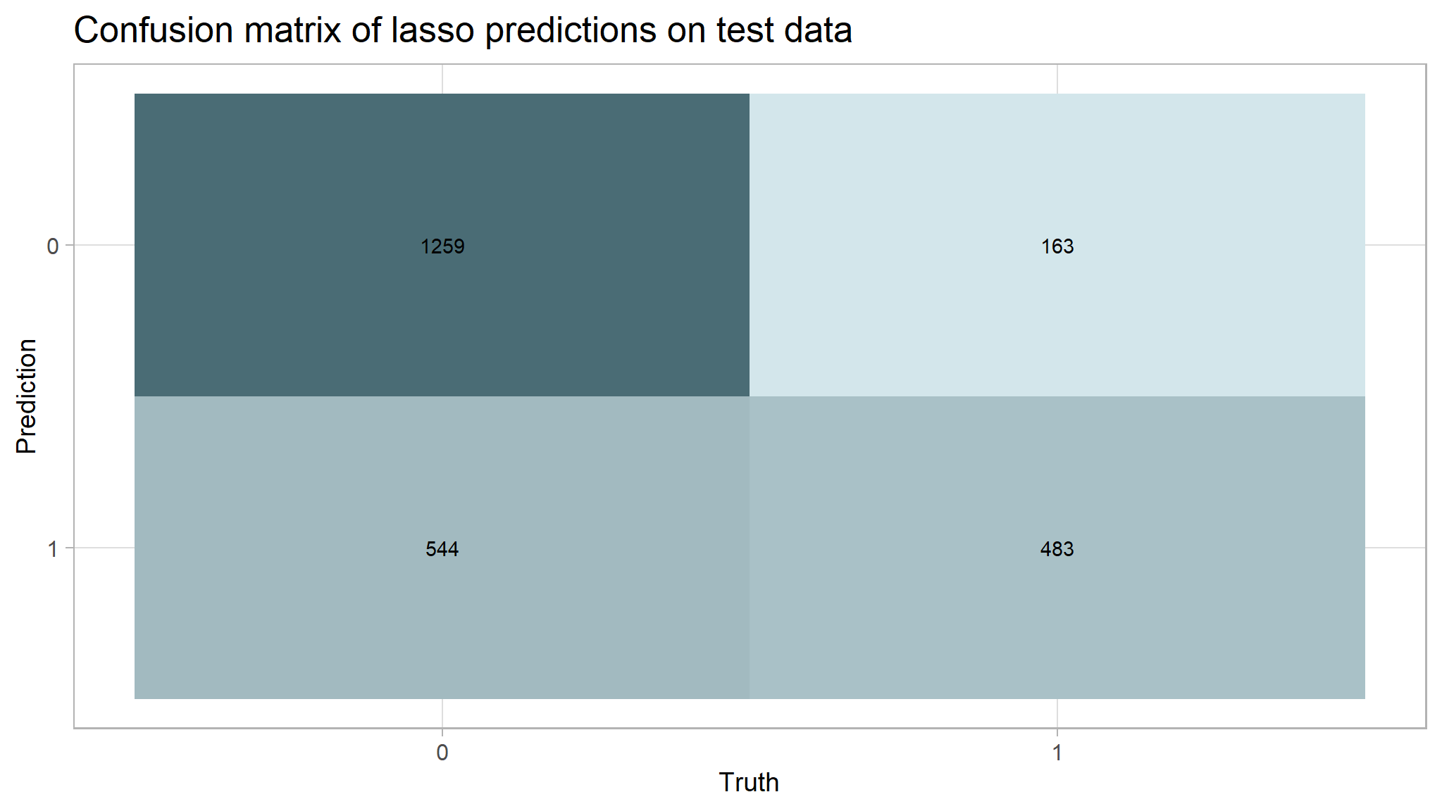


# Calculate rates of tru pos, false neg. etc. from the confusion matrix
TP_las <- cm_lasso$table[2, 2]
FP_las <- cm_lasso$table[2, 1]
TN_las <- cm_lasso$table[1, 1]
FN_las <- cm_lasso$table[1, 2]
TPR_las <- TP_las / (TP_las + FN_las)  # True Positive Rate
FPR_las <- FP_las / (FP_las + TN_las)  # False Positive Rate
TNR_las <- TN_las / (TN_las + FP_las)  # True Negative Rate
FNR_las <- FN_las / (TP_las + FN_las)  # False Negative Rate

# Create cm df to hold all false pos, etc. metrics
lasso_cm_vec <- c(TPR_las, FPR_las, TNR_las, FNR_las)
row_names <- c("True positive rate", "False positive rate", "True negative rate", "False negative rate")
cm_df <- bind_cols(Metric = row_names, Lasso = lasso_cm_vec)

The accuracy for the lasso model was 0.711 which is slightly lower than our dummy classifier that had an accuracy of 0.736. This model had an AUC of 0.79.

K-Nearest Neighbors

set.seed(123)

# Define the KNN model with tuning
knn_spec_tune <- nearest_neighbor(neighbors = tune()) %>% # tune k
  set_mode("classification") %>% 
  set_engine("kknn")

# Define a new workflow
wf_knn_tune <- workflow() %>% 
  add_model(knn_spec_tune) %>% 
  add_recipe(boost_recipe)
    
# Fit the workflow on the predefined folds and hyperparameters
fit_knn_cv <- wf_knn_tune %>% 
  tune_grid( 
    fish_cv, 
    grid = data.frame(neighbors = c(1,5,10,15,seq(20,200,10))))

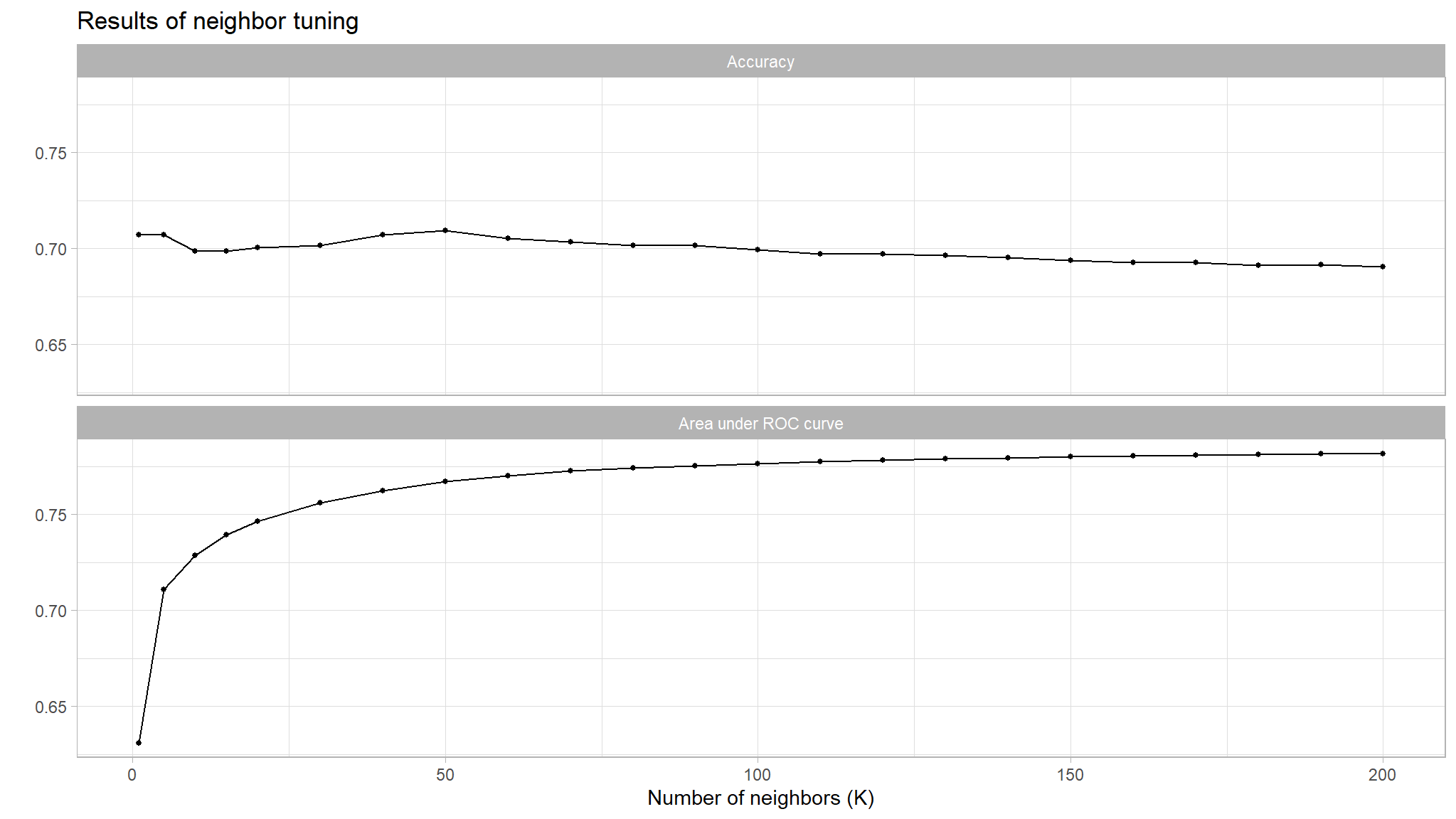
# Use autoplot() to examine how different parameter configurations relate to accuracy
autoplot(fit_knn_cv) +
  theme_light() +
  labs(
    x = "Number of neighbors (K)",
    title = "Results of neighbor tuning"
  ) +
  theme(
    legend.position = "none",
    panel.background = element_blank(),
    plot.background = element_blank()
  ) +
  facet_wrap(
    ~.metric,
    nrow = 2,
    labeller = labeller(.metric = c("accuracy" = "Accuracy", "roc_auc" = "Area under ROC curve"))
  )


# View table
fit_knn_cv %>%
  tune::show_best(metric = "roc_auc") %>%
  slice_head(n = 5) %>% 
  kable(caption = "Performance of the best models and the associated estimates for the number of neighbors parameter values.")

Performance of the best models and the associated estimates for the number of neighbors parameter values.
neighbors	.metric	.estimator	mean	n	std_err	.config
200	roc_auc	binary	0.7817082	10	0.0061542	Preprocessor1_Model23
190	roc_auc	binary	0.7814088	10	0.0061576	Preprocessor1_Model22
180	roc_auc	binary	0.7810887	10	0.0061389	Preprocessor1_Model21
170	roc_auc	binary	0.7808321	10	0.0061081	Preprocessor1_Model20
160	roc_auc	binary	0.7804127	10	0.0060630	Preprocessor1_Model19


# Select the model with the highest auc
best_knn <- fit_knn_cv %>%
  select_best("roc_auc")

# The final workflow for our KNN model
final_knn_wf <-
  wf_knn_tune %>% 
  finalize_workflow(best_knn)

# Use last_fit() approach to apply model to test data
final_knn_fit <- last_fit(final_knn_wf, auto_split)

# Collect metrics on the test data
tibble_knn <- final_knn_fit %>% collect_metrics()
tibble_knn %>% 
  kable(caption = "Accuracy and area under the receiver operator curve of the final fit.")

Accuracy and area under the receiver operator curve of the final fit.
.metric	.estimator	.estimate	.config
accuracy	binary	0.6831360	Preprocessor1_Model1
roc_auc	binary	0.7835565	Preprocessor1_Model1


# Store accuracy and AUC
final_knn_accuracy <- tibble_knn %>%
  filter(.metric == "accuracy") %>%
  pull(.estimate)
final_knn_auc <- tibble_knn %>%
  filter(.metric == "roc_auc") %>%
  pull(.estimate)

# Bind predictions and original data
knn_test_rs <- cbind(test, final_knn_fit$.predictions)[, -16]

# Compute a confusion matrix
cm_knn <- knn_test_rs %>% yardstick::conf_mat(truth = target_flag, estimate = .pred_class) 

# Create the confusion matrix heatmap plot
autoplot(cm_knn, type = "heatmap") +
  custom_palette +
  theme(
    axis.text.x = element_text(size = 12),
    axis.text.y = element_text(size = 12),
    axis.title = element_text(size = 14),
    panel.background = element_blank(),
    plot.background = element_blank()
  ) +
  labs(title = "Confusion matrix of knn predictions on test data")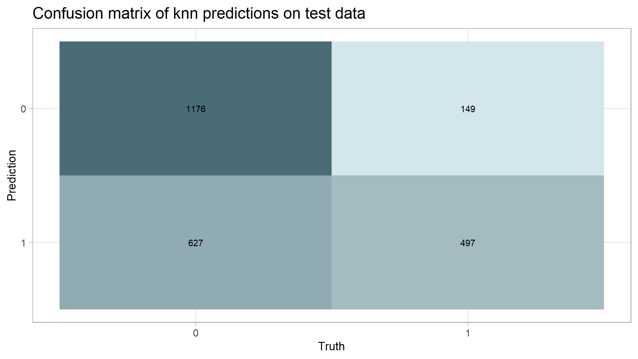



# Calculate rates from the confusion matrix
TP_knn <- cm_knn$table[2, 2]
FP_knn <- cm_knn$table[2, 1]
TN_knn <- cm_knn$table[1, 1]
FN_knn <- cm_knn$table[1, 2]
TPR_knn <- TP_knn / (TP_knn + FN_knn)  # True Positive Rate
FPR_knn <- FP_knn / (FP_knn + TN_knn)  # False Positive Rate
TNR_knn <- TN_knn / (TN_knn + FP_knn)  # True Negative Rate
FNR_knn <- FN_knn / (TP_knn + FN_knn)  # False Negative Rate

# Add rates to cm df
knn_cm_vec <- c(TPR_knn, FPR_knn, TNR_knn, FNR_knn)
cm_df$KNN <- knn_cm_vec

The k-nearest neighbors model had nearly the same accuracy at predicting threat status than the dummy classifier. The accuracy of the model was 0.683. This model had an AUC of 0.784 which is better than the lasso model.

Decision Tree

# Tell the model that we are tuning hyperparams
tree_spec_tune <- decision_tree(
  cost_complexity = tune(),
  tree_depth = tune(),
  min_n = tune()) %>% 
  set_engine("rpart") %>% 
  set_mode("classification")

# Set up grid
tree_grid <- grid_regular(cost_complexity(), tree_depth(), min_n(), levels = 5)

# Check grid
#tree_grid 

# Define a workflow with the recipe and specification
wf_tree_tune <- workflow() %>% 
  add_recipe(boost_recipe) %>% 
  add_model(tree_spec_tune)

doParallel::registerDoParallel(cores = 3) #build trees in parallel

# Tune
tree_rs <- tune_grid(
  wf_tree_tune,
  target_flag~.,
  resamples = fish_cv,
  grid = tree_grid,
  metrics = metric_set(roc_auc)
)

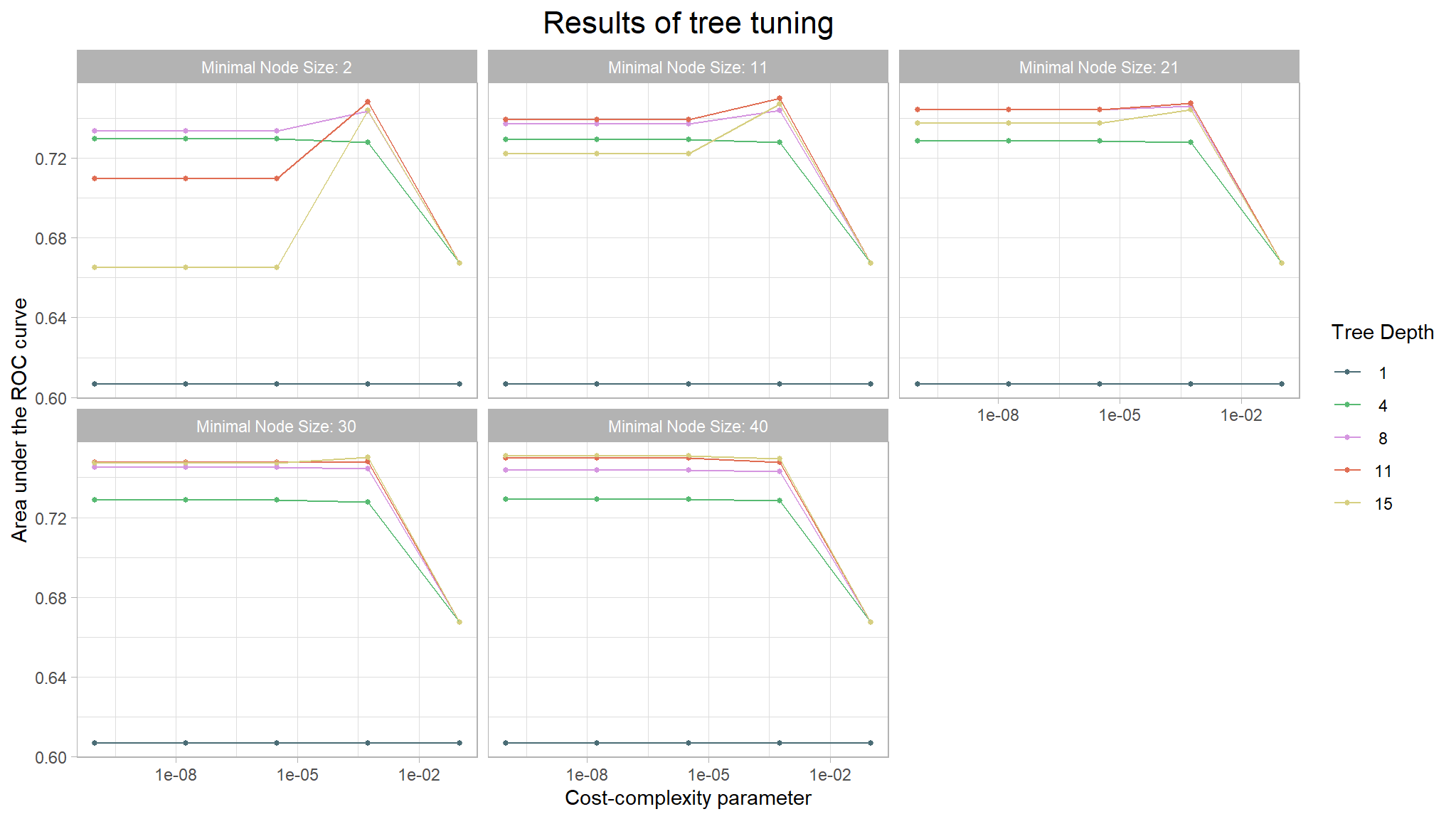
# Use autoplot() to examine how different parameter configurations relate to auc
autoplot(tree_rs) + 
  theme_light() +
  scale_color_manual(values = c("#4a6c75", "#57ba72", "#d596e0", "#e06d53", "#d6cf81")) + 
  labs(x = "Cost-complexity parameter",
       y = "Area under the ROC curve",
       title = "Results of tree tuning") +
  theme(
    plot.title = element_text(size = 16, hjust = 0.5),
    panel.background = element_blank(),
    plot.background = element_blank()
  )


# View table
tree_rs %>%
  tune::show_best(metric = "roc_auc") %>%
  slice_head(n = 5) %>% 
  kable(caption = "Performance of the best models and the associated estimates for the tuned tree parameter values.")

Performance of the best models and the associated estimates for the tuned tree parameter values.
cost_complexity	tree_depth	min_n	.metric	.estimator	mean	n	std_err	.config
0.0000000	15	40	roc_auc	binary	0.7507165	10	0.0041181	Preprocessor1_Model121
0.0000000	15	40	roc_auc	binary	0.7507165	10	0.0041181	Preprocessor1_Model122
0.0000032	15	40	roc_auc	binary	0.7507165	10	0.0041181	Preprocessor1_Model123
0.0005623	11	11	roc_auc	binary	0.7501208	10	0.0057635	Preprocessor1_Model044
0.0005623	15	30	roc_auc	binary	0.7499908	10	0.0045924	Preprocessor1_Model099


# Finalize the model specs with the best hyperparameter result
final_tree <- finalize_model(tree_spec_tune, select_best(tree_rs))

# Final fit to test data 
final_tree_fit <- last_fit(final_tree, target_flag~., auto_split) # does training fit then final prediction as well

# Collect metrics from fit
tibble_tree <- final_tree_fit %>% collect_metrics()
tibble_tree %>% kable(caption = "Accuracy and area under ther receiver operator curve of the final fit.")

Accuracy and area under ther receiver operator curve of the final fit.
.metric	.estimator	.estimate	.config
accuracy	binary	1	Preprocessor1_Model1
roc_auc	binary	1	Preprocessor1_Model1


# Store accuracy and auc metrics
final_tree_accuracy <- tibble_tree %>%
  filter(.metric == "accuracy") %>%
  pull(.estimate)

final_tree_auc <- tibble_tree %>%
  filter(.metric == "roc_auc") %>%
  pull(.estimate)

# Bind predictions and original data
tree_test_rs <- cbind(test, final_tree_fit$.predictions)[, -16]

# Compute a confusion matrix
cm_tree <- tree_test_rs %>% yardstick::conf_mat(truth = target_flag, estimate = .pred_class) 

custom_palette <- scale_fill_gradient(
  high = "#07193b",  
  low = "#4a6c75"  
)
# Create the confusion matrix heatmap plot
autoplot(cm_tree, type = "heatmap") +
  custom_palette +
  theme(
    axis.text.x = element_text(size = 12),
    axis.text.y = element_text(size = 12),
    axis.title = element_text(size = 14),
    panel.background = element_blank(),
    plot.background = element_blank()
  ) +
  labs(title = "Confusion matrix of decision tree predictions on test data")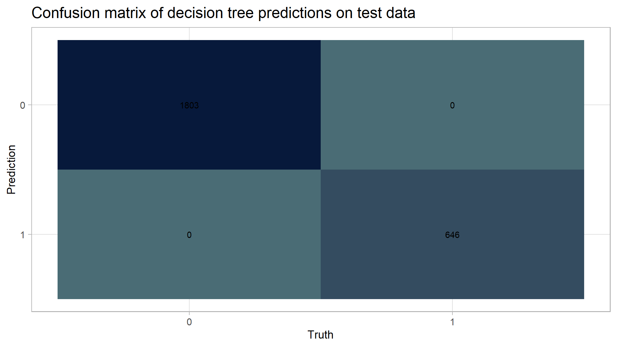



# Calculate rates from the confusion matrix
TP_tree <- cm_tree$table[2, 2]
FP_tree <- cm_tree$table[2, 1]
TN_tree <- cm_tree$table[1, 1]
FN_tree <- cm_tree$table[1, 2]
TPR_tree <- TP_tree / (TP_tree + FN_tree)  # True Positive Rate
FPR_tree <- FP_tree / (FP_tree + TN_tree)  # False Positive Rate
TNR_tree <- TN_tree / (TN_tree + FP_tree)  # True Negative Rate
FNR_tree <- FN_tree / (TP_tree + FN_tree)  # False Negative Rate

# Add rates to cm df
tree_cm_vec <- c(TPR_tree, FPR_tree, TNR_tree, FNR_tree)
cm_df$DecisionTree <- tree_cm_vec

The decision tree model had a higher accuracy at predicting risk than the dummy classifier. The accuracy of the decision tree was 1. The AUC is 1 which is lower than the lasso model and the knn model.

Model Results

Model selection

I want to compare accuracy and area under the curve of all models created.

# Name models in vec
models <- c("Dummy", "Lasso", "KNN","DecisionTree")

# Create accuracy vec
accuracy <- c(dummy, final_lasso_accuracy, final_knn_accuracy,final_tree_accuracy)

# Make df
accuracy_df <- data.frame(models, accuracy)

# Create a factor with the desired order for models
accuracy_df$models <- factor(accuracy_df$models, levels = c("Dummy", "Lasso", "KNN","DecisionTree"))

# Create the plot
ggplot(accuracy_df, aes(x = models, y = accuracy)) +
  geom_col(fill = "#4a6c75") +
  theme_minimal() +
  labs(title = "Accuracy was similar across all models",
    x = "Model",        
    y = "Accuracy") +
  geom_text(aes(label = round(accuracy, 3)), vjust = -0.5) +
  theme(plot.background = element_blank(),
        panel.background = element_blank())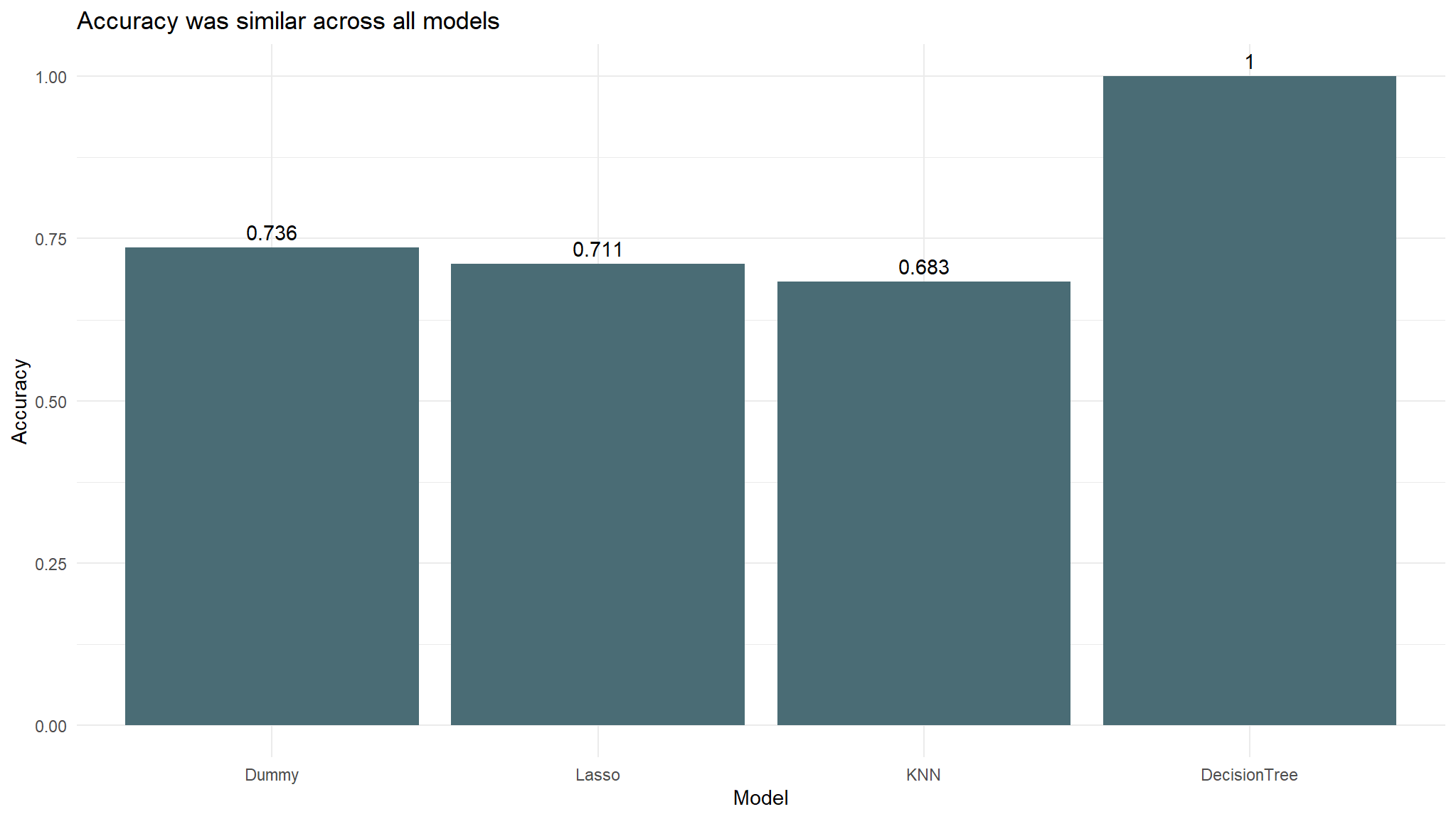


# Create auc vec
auc <- c(final_lasso_auc, final_knn_auc,final_tree_auc)

# Make df
auc_df <- data.frame(models[-1], auc)

# Create a factor with the desired order for models
auc_df$models <- factor(auc_df$models, levels = c("Lasso", "KNN" ,"DecisionTree"))

ggplot(auc_df, aes(x = models, y = auc)) +
  geom_col(fill = "#4a6c75") +
  theme_minimal() +
  labs(title = "Logistic lasso was the highest performing model",
    x = NULL,        
    y = "Area under ROC curve") +
    geom_text(aes(label = round(auc, 3)), vjust = -0.5) +
  theme(plot.background = element_blank(),
        panel.background = element_blank())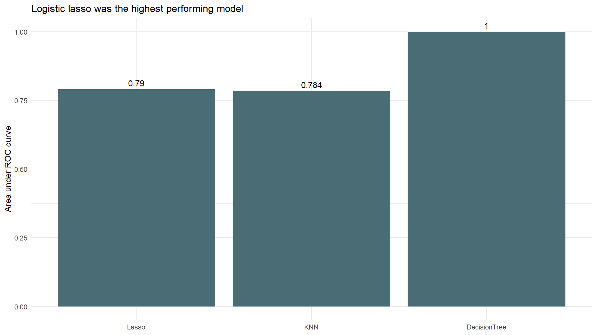

the accuracies between models don’t vary much. It is difficult to get much more accurate than always choosing not threatened (the dummy classifier) because that already has an accuracy of 0.736.

I also want to compare the confusion matrix values of each model.

# Print table
cm_df %>% 
  kable()

Metric	Lasso	KNN	DecisionTree
True positive rate	0.7476780	0.7693498	1
False positive rate	0.3017194	0.3477537	0
True negative rate	0.6982806	0.6522463	1
False negative rate	0.2523220	0.2306502	0




# Plot the true pos etc rates
cm_df %>% 
  pivot_longer(cols = Lasso:DecisionTree) %>% 
  ggplot(aes(x = name, y = value, fill = Metric)) +
  geom_col() +
  theme_minimal() +
  labs(x = NULL,
       y = "Value",
       title = "Rates of true positive, true negative, etc. for each model")  +
  theme(plot.background = element_blank(),
        panel.background = element_blank()) +
  ggthemes::scale_fill_tableau()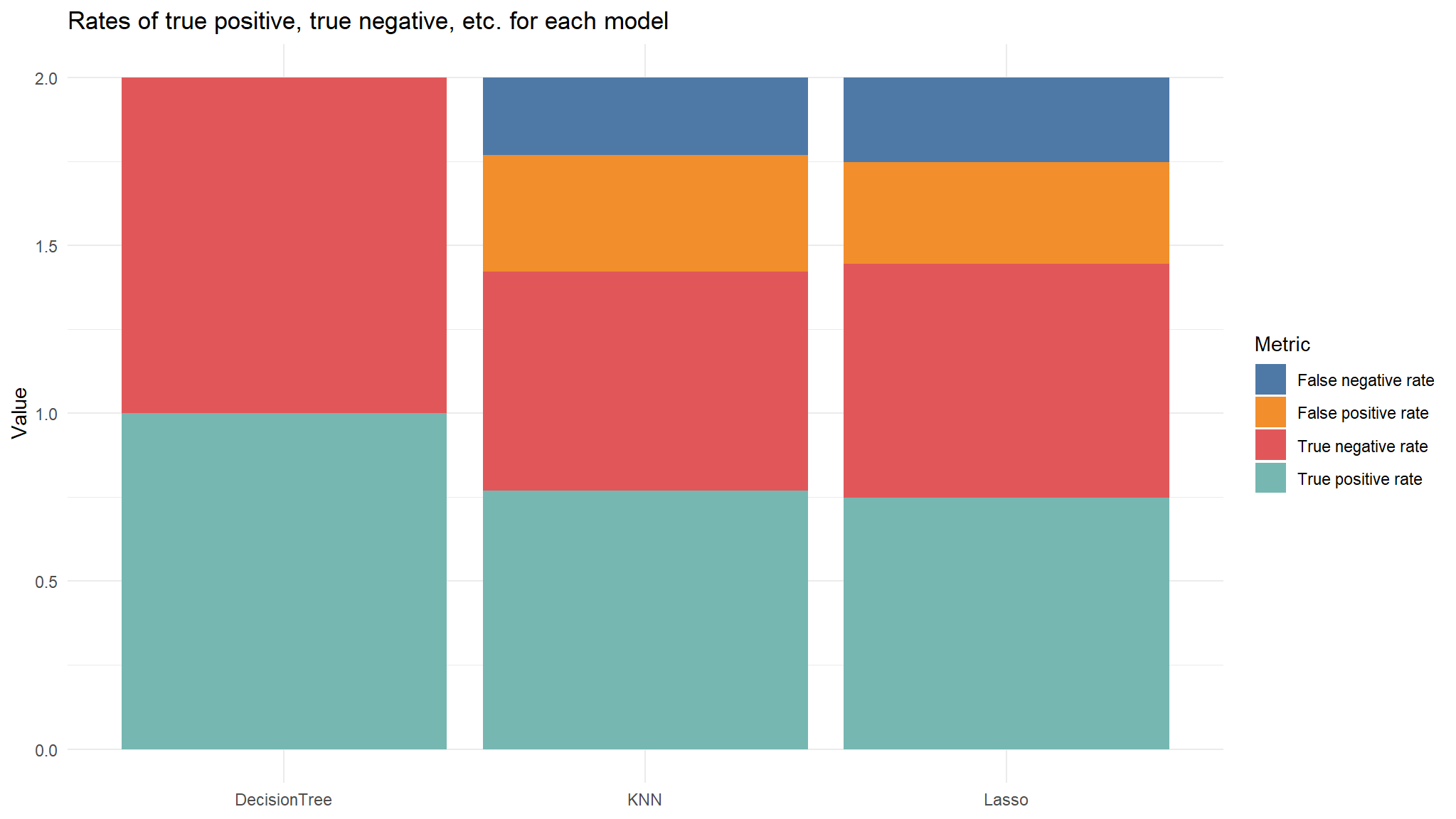

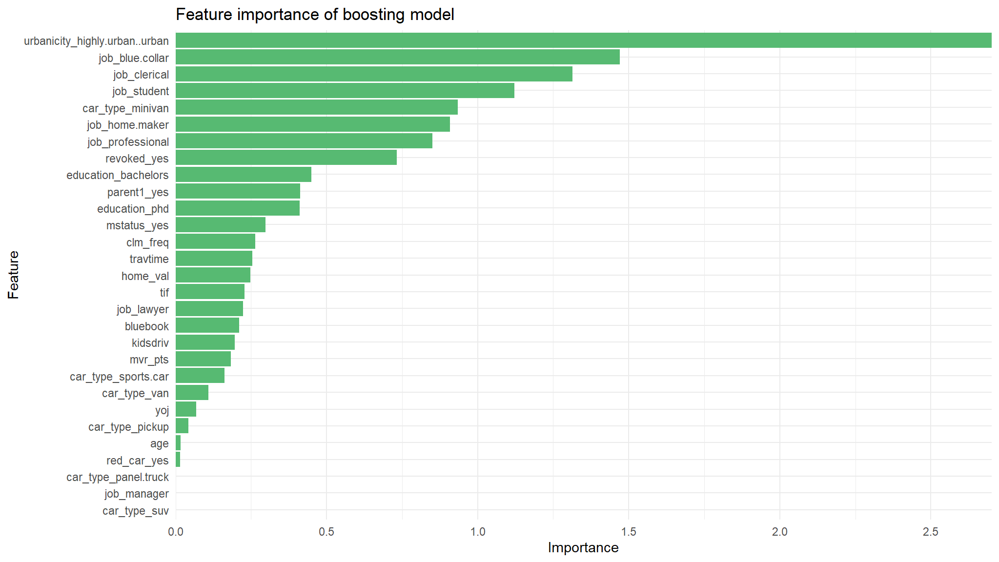
Variable Importance

I want to look at the variable importance of the most successful model, lasso logistic.

# Variable importance
var_imp_boost <- final_l_wf %>% 
  fit(train) %>% 
  pull_workflow_fit() %>%
  vi() %>%
  mutate(
    Importance = abs(Importance),
    Variable = fct_reorder(Variable, Importance))
var_imp_boost %>% 
  ggplot(aes(x = Importance, y = Variable)) +
  geom_col(fill = "#57ba72") +
  theme_minimal() +
  scale_x_continuous(expand = c(0, 0)) +
  labs(y = "Feature",
       x = "Importance",
       title = "Feature importance of boosting model") +
  theme(plot.background = element_blank(),
        panel.background = element_blank())