Recipe type classification
1. Data Validation
This data set has 947 rows, 8 columns. I have validated all variables and I have made several changes after validation: remove rows with null values in calories, carbohydrate, sugar, protein and replace null values in high_traffic with “Low”.
- recipe: 947 unique identifiers without missing values (895 after dataset cleaning). No cleaning is needed.
- calories: 895 non-null values. I fill 52 missed values with the mean value.
- carbohydrate: 895 non-null values. I fill 52 missed values with the mean value.
- sugar: 895 non-null values. I fill 52 missed values with the mean value.
- protein: 895 non-null values. I fill 52 missed values with the mean value.
- category: 11 unique values without missing values, whereas there were 10 values in the description. The extra valie is ‘Chicken Breast’. I united it with the ‘Chicken’ value.
- servings: 6 unique values without missing values. By description, it should be numeric variable, but now it’s character. Has two extra values: ‘4 as a snack’ and ‘6 as a snack’. I united them with ‘4’ and ‘6’ and changed the column’s type to integer.
- high_traffic: only 1 non-null value (“High”). Replaced null values with “Low”.
load in necessary packages
overview of the data set
recipe |
calories |
carbohydrate |
sugar |
protein |
category |
servings |
high_traffic |
|---|---|---|---|---|---|---|---|
1 |
Pork |
6 |
High |
||||
2 |
35.48 |
38.56 |
0.66 |
0.92 |
Potato |
4 |
High |
3 |
914.28 |
42.68 |
3.09 |
2.88 |
Breakfast |
1 |
|
4 |
97.03 |
30.56 |
38.63 |
0.02 |
Beverages |
4 |
High |
5 |
27.05 |
1.85 |
0.80 |
0.53 |
Beverages |
4 |
|
6 |
691.15 |
3.46 |
1.65 |
53.93 |
One Dish Meal |
2 |
High |
look at the missing values
- validating the dataset for missing values
data wrangling and exploration
- There are only 2 and 1 recipes of 4 as a snack and 6 as a snack servings, so I’ll rename them to “4” and “6” for simplicity and convert to numerical.
- replace null values of high_traffic with Low
- chicken breast turned to just chicken
inspect the data for the new changes
Servings
category
High Traffic
high_traffic |
n |
percent |
|---|---|---|
High |
574 |
0.6061246 |
low |
373 |
0.3938754 |
- replace missing values with mean
recipe_data_new<-recipe_data_new |>
  mutate(sugar = replace_na(sugar,mean(sugar,na.rm=T)),
         calories = replace_na(calories,mean(calories,na.rm=T)),
         protein = replace_na(protein,mean(protein,na.rm=T)),
         carbohydrate =replace_na(carbohydrate,mean(carbohydrate,na.rm=T)))
recipe_data_new|> head() |>  flextable()
recipe |
calories |
carbohydrate |
sugar |
protein |
category |
servings |
high_traffic |
|---|---|---|---|---|---|---|---|
1 |
435.9392 |
35.06968 |
9.046547 |
24.1493 |
Pork |
6 |
High |
2 |
35.4800 |
38.56000 |
0.660000 |
0.9200 |
Potato |
4 |
High |
3 |
914.2800 |
42.68000 |
3.090000 |
2.8800 |
Breakfast |
1 |
low |
4 |
97.0300 |
30.56000 |
38.630000 |
0.0200 |
Beverages |
4 |
High |
5 |
27.0500 |
1.85000 |
0.800000 |
0.5300 |
Beverages |
4 |
low |
6 |
691.1500 |
3.46000 |
1.650000 |
53.9300 |
One Dish Meal |
2 |
High |
Data visualisation
ggplot(recipe_data_new) +
  aes(x=factor(servings)) +
  aes(fill=high_traffic) +
  geom_bar(position="dodge",
       color="black") +
  geom_text(aes(label=after_stat(count)),
     stat='count',
     position=position_dodge(1.0),
     vjust= -0.5,
size=3) 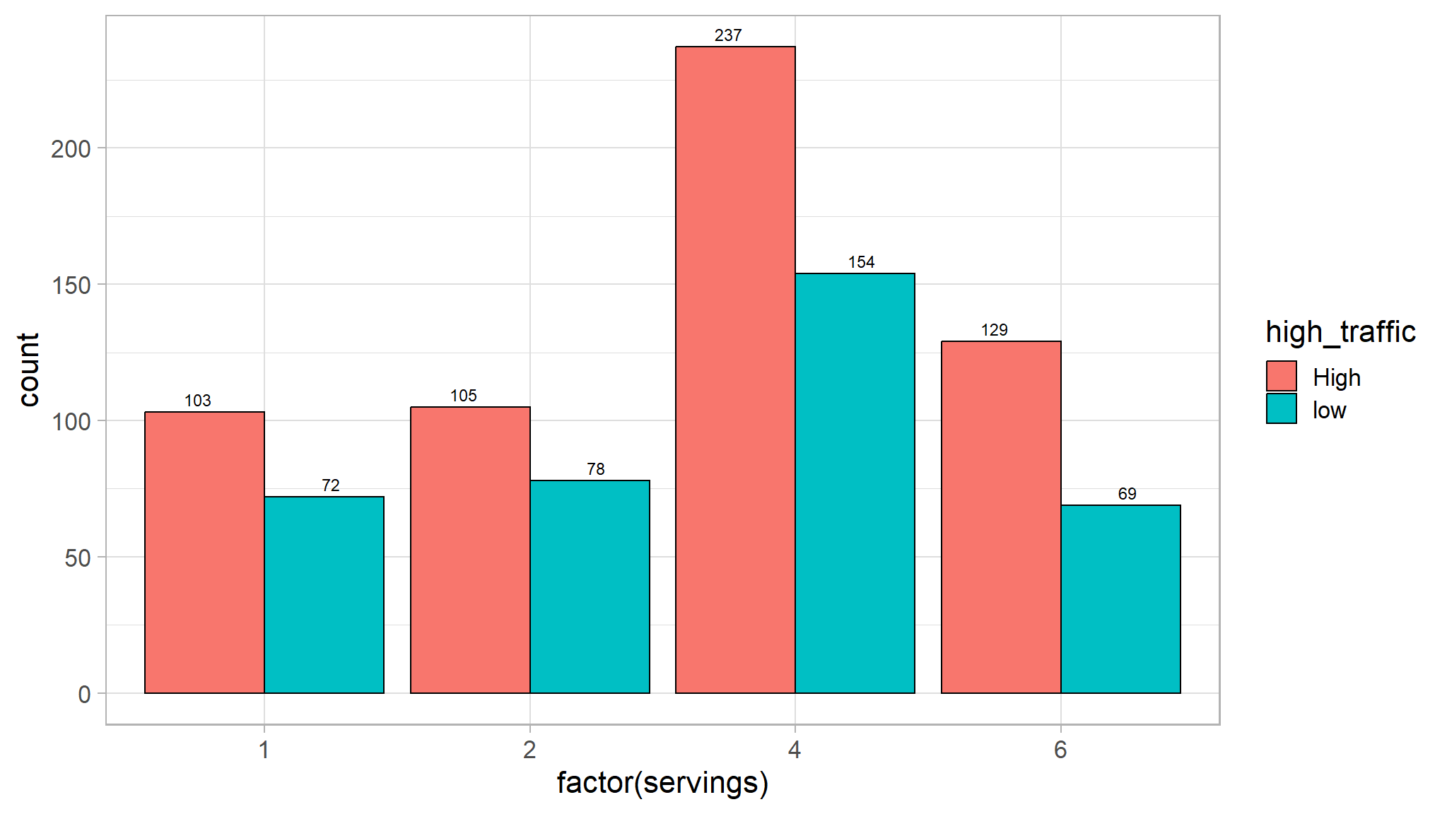
- this feature doesn’t have a big influence on target variable because recipes with high traffic are are many for each servings as compared to the those in with low traffic.
ggplot(recipe_data_new) +
  aes(x=category) +
  aes(fill=high_traffic) +
  geom_bar(position="dodge",
       color="black") +
  geom_text(aes(label=after_stat(count)),
     stat='count',
     position=position_dodge(1.0),
     vjust= -0.5,
     size=3)+
  theme(legend.position = 'none')+
  theme(axis.text.x = element_text(angle = 45, hjust = 1))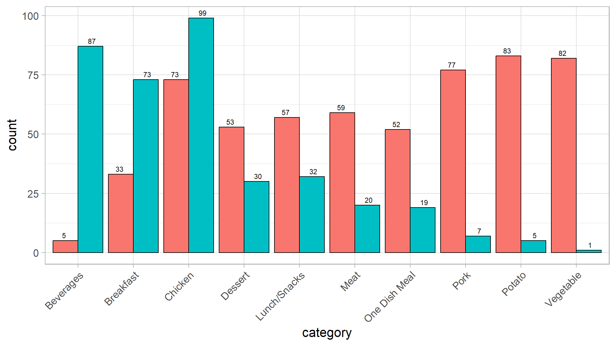
- Potato, Pork and Vegetable categories have a lot more recipes with high traffic than with low traffic.
- One Dish Meal, Lunch/Snacks, Meat, Dessert categories have just more recipes with high traffic than with low traffic.
Correlations
## select only numeric values
cor_data<-recipe_data_new %>%
  keep(is.numeric)
## create a correlation matrix
corl<-cor(cor_data)
corrplot::corrplot(corl,method="color",addCoef.col = "black")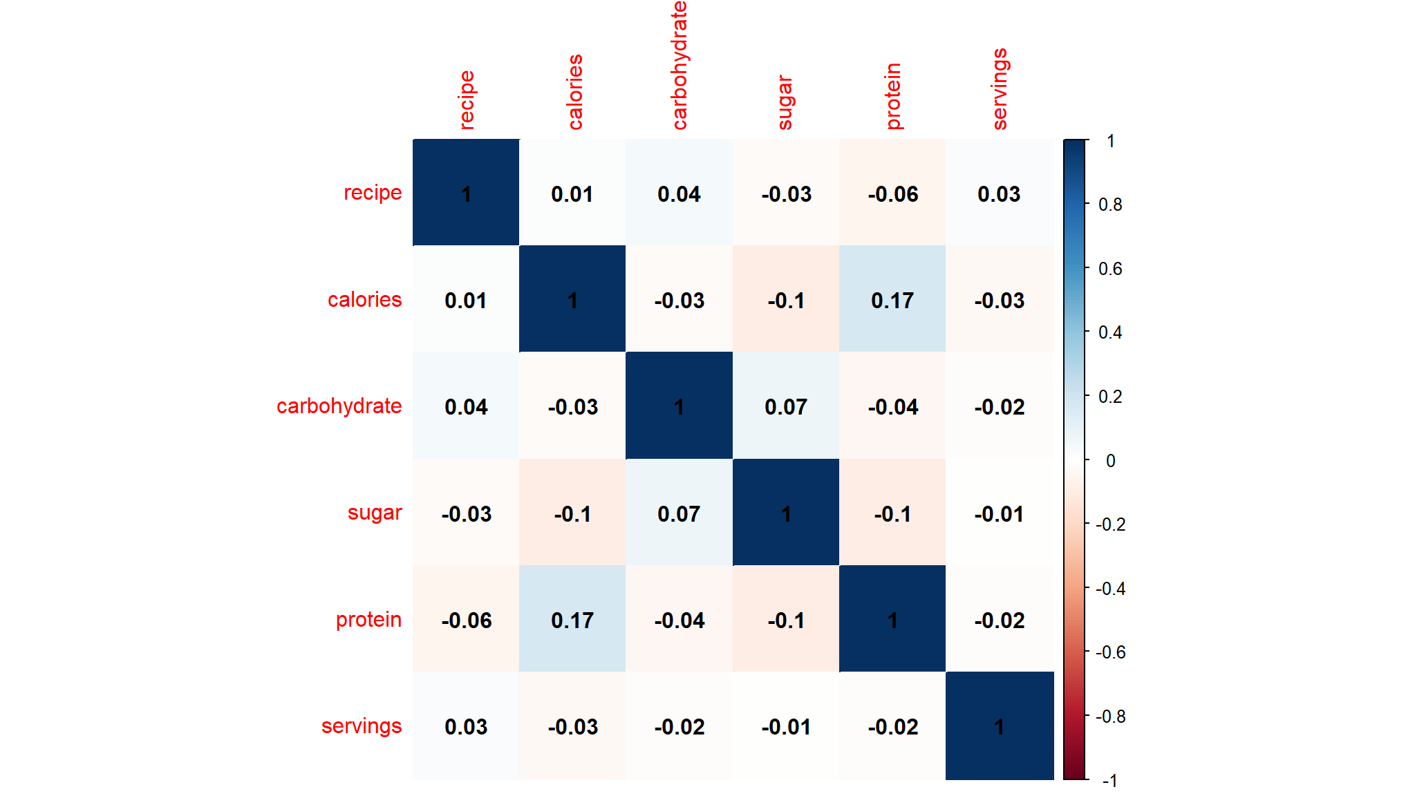
- the heatmap above suggests that there is little to no linear negative relationship in 5 variables
- calories, carbohydrate, sugar, protein, servings. All values are close to 0, so we can say there is a weak relationship between the variables.
- individual plots of both nutrients are shown in the facets below
- looking if there outliers in the nutrients
recipe_data_new |>
  select(sugar,calories,carbohydrate,protein) |>
  gather() |>
  ggplot(aes(key,value,fill=key)) +
  ggthemes::scale_fill_tableau()+
  geom_boxplot() +
  facet_wrap(~key,scales="free")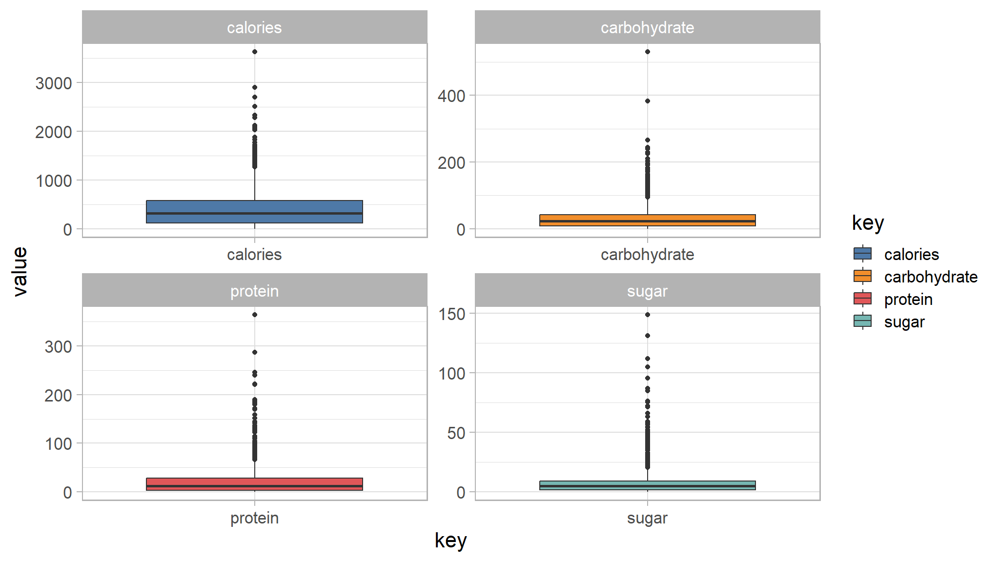
Histogram
recipe_data_new |>
  select(sugar,calories,carbohydrate,protein) |>
  gather() |>
  ggplot(aes(value,fill=key)) +
  ggthemes::scale_fill_tableau()+
  geom_histogram() +
  facet_wrap(~key,scales="free")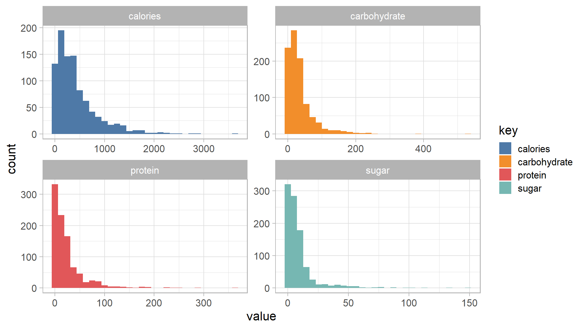
- from the histograms above ,both nutrients are seen to be right skewed
let’s visually inspect single variables
- look at calories
recipe_data_new |>
  ggplot(aes(calories)) +
  ggthemes::scale_fill_tableau()+
geom_histogram() 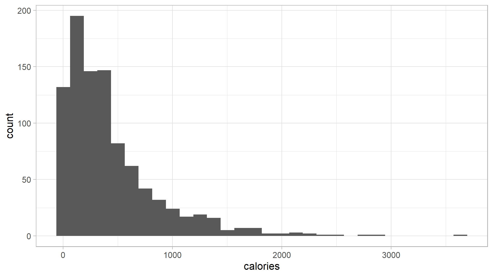
- the data for calories is right skewed as seen from the histogram
recipe_data_new |>
  ggplot(aes(x=1,y=calories)) +
  ggthemes::scale_fill_tableau()+
geom_boxplot(outlier.colour="red") 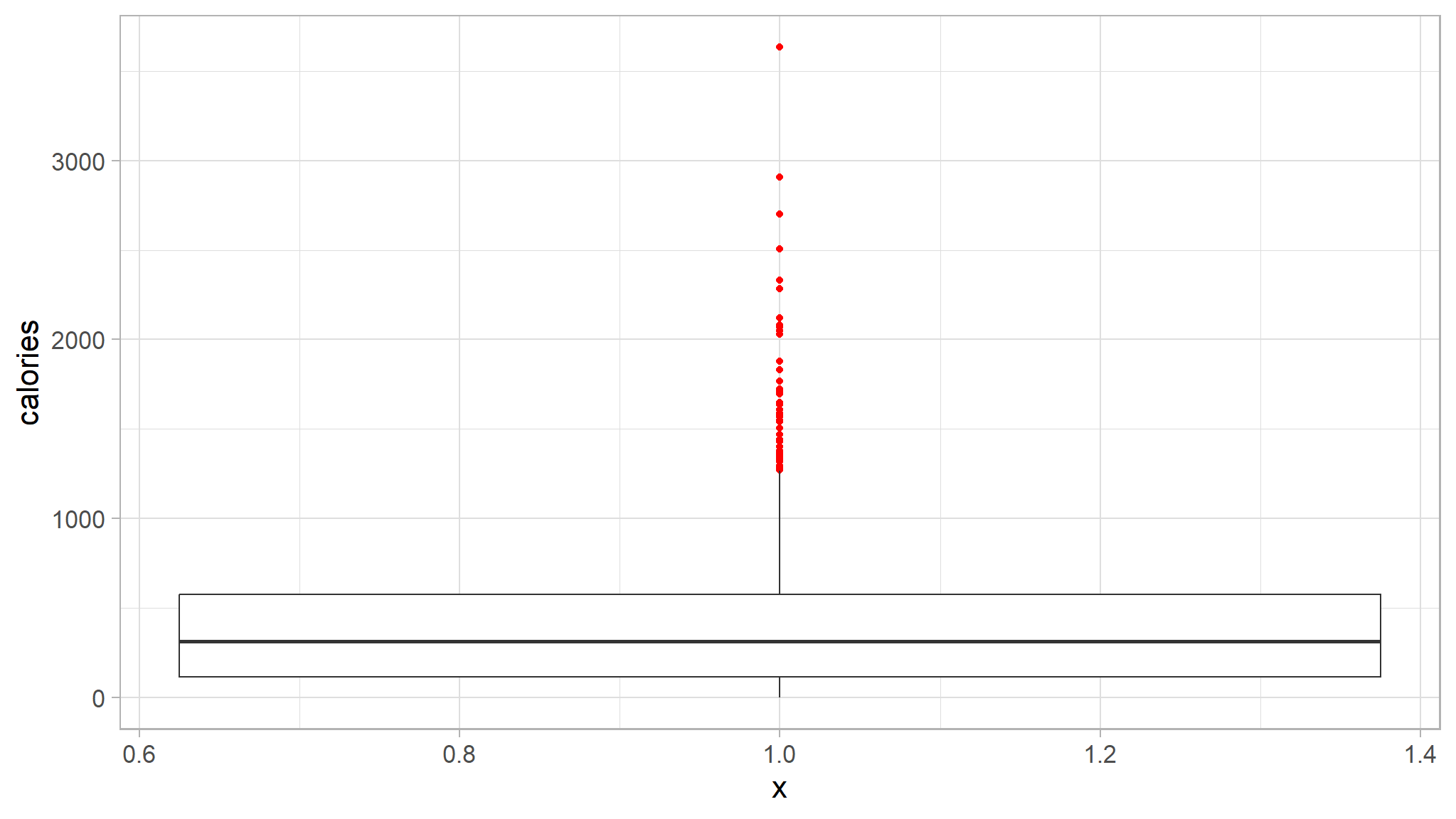
- the points in red indicate potential outliers in the data
recipe_data_new |>
  select(sugar,calories,carbohydrate,protein,high_traffic) |>
  gather("key","value",-high_traffic) |>
  ggplot(aes(value,color=high_traffic)) +
  ggthemes::scale_fill_tableau()+
  geom_density() +
  facet_wrap(~key,scales="free")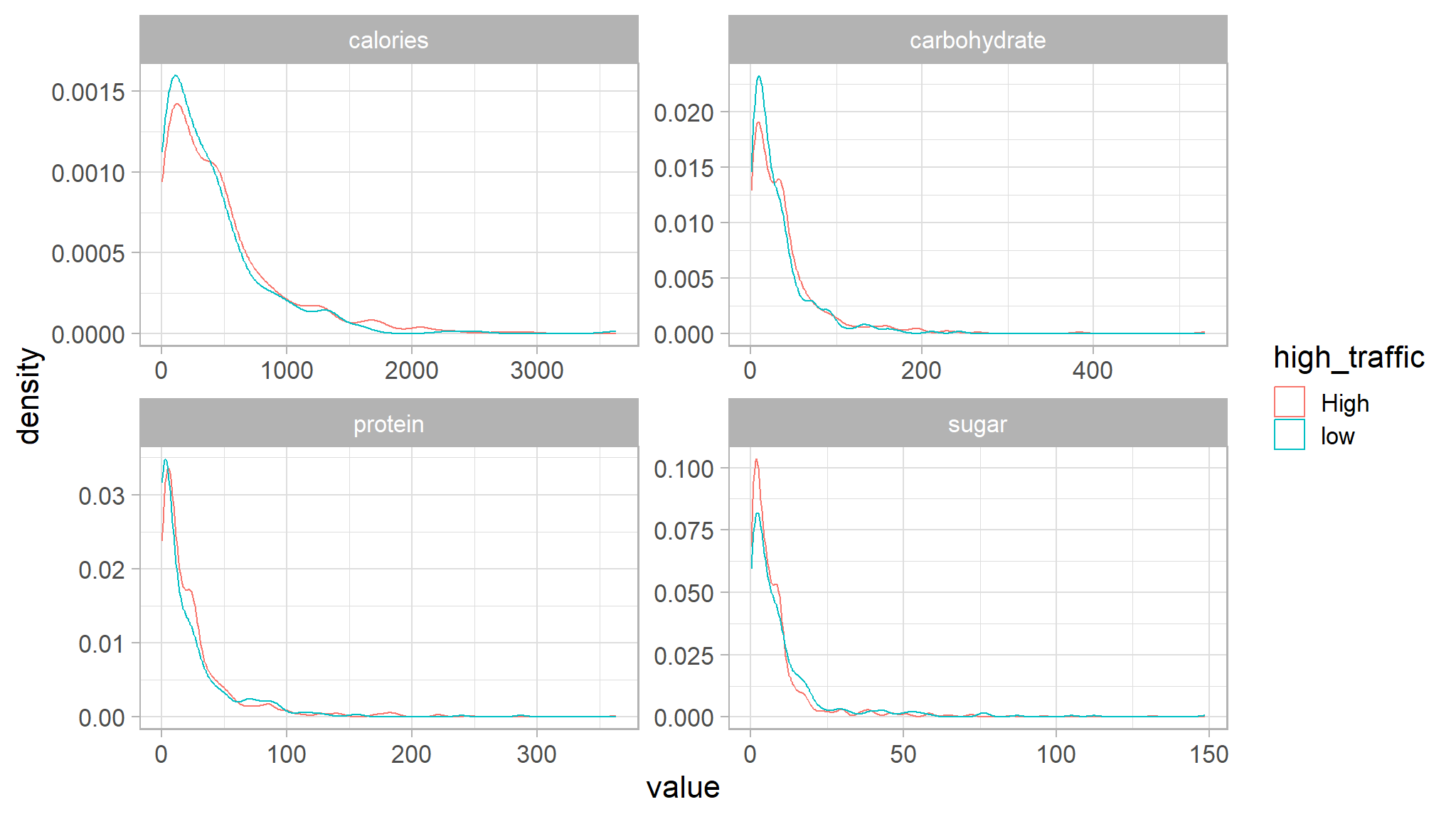
the density plots shows that there are no significant depedencies of the traffic and the following numerical features: calories, carbohydrate, protein, sugar, servings.
Modeling data
#> Training cases: 662
#> Test cases: 285
#> # A tibble: 5 × 7
#>   calories carbohydrate sugar protein category     servings high_traffic
#>      <dbl>        <dbl> <dbl>   <dbl> <chr>           <dbl> <fct>
#> 1   960.           4.4  44.5    12.1  Dessert             1 0
#> 2   189.           9.54  6.47    0.34 Beverages           6 0
#> 3   248.          44.7   2.64   19.9  Chicken             1 1
#> 4     6.23        56.4   5.6     2.12 Lunch/Snacks        6 1
#> 5    81.0          0.35  1.27    1.19 Beverages           4 0
Train and Evaluate a Binary Classification Model
OK, now we’re ready to train our model by fitting the training features to the training labels (high_trafffic).
Preprocess the data for modelling
- normalize all numerical features
- turn categorical data to numerical data by creating dummy variables
recipe_data_recipe <- recipe(high_traffic ~ ., data = recipe_data_train)|>
  step_normalize(all_numeric_predictors())|>
  step_dummy(all_nominal_predictors())
fit the model
# Redefine the model specification
logreg_spec <- logistic_reg()|>
  set_engine("glm")|>
  set_mode("classification")

# Bundle the recipe and model specification
lr_wf <- workflow()|>
  add_recipe(recipe_data_recipe)|>
  add_model(logreg_spec)

# Print the workflow
lr_wf
#> ══ Workflow ════════════════════════════════════════════════════════════════════
#> Preprocessor: Recipe
#> Model: logistic_reg()
#>
#> ── Preprocessor ────────────────────────────────────────────────────────────────
#> 2 Recipe Steps
#>
#> • step_normalize()
#> • step_dummy()
#>
#> ── Model ───────────────────────────────────────────────────────────────────────
#> Logistic Regression Model Specification (classification)
#>
#> Computational engine: glm
# Fit a workflow object
lr_wf_fit <- lr_wf|>
fit(data = recipe_data_train)
# Print wf object
lr_wf_fit
#> ══ Workflow [trained] ══════════════════════════════════════════════════════════
#> Preprocessor: Recipe
#> Model: logistic_reg()
#>
#> ── Preprocessor ────────────────────────────────────────────────────────────────
#> 2 Recipe Steps
#>
#> • step_normalize()
#> • step_dummy()
#>
#> ── Model ───────────────────────────────────────────────────────────────────────
#>
#> Call: stats::glm(formula = ..y ~ ., family = stats::binomial, data = data)
#>
#> Coefficients:
#> (Intercept) calories carbohydrate
#> -3.17385 0.05534 0.03697
#> sugar protein servings
#> -0.06993 0.02482 -0.02061
#> category_Breakfast category_Chicken category_Dessert
#> 2.42197 2.95913 3.81616
#> category_Lunch.Snacks category_Meat category_One.Dish.Meal
#> 3.53970 4.33127 3.92688
#> category_Pork category_Potato category_Vegetable
#> 6.07030 6.10736 7.28483
#>
#> Degrees of Freedom: 661 Total (i.e. Null); 647 Residual
#> Null Deviance: 880.6
#> Residual Deviance: 627.8 AIC: 657.8lr_fitted_add <- lr_wf_fit|>
extract_fit_parsnip()|>
tidy() |>
mutate(Significance = ifelse(p.value < 0.05,
"Significant", "Insignificant"))|>
arrange(desc(p.value))
#Create a ggplot object to visualise significance
plot <- lr_fitted_add|>
ggplot(mapping = aes(x=term, y=p.value, fill=Significance)) +
geom_col() +
ggthemes::scale_fill_tableau() +
theme(axis.text.x = element_text(face="bold",
color="#0070BA",
size=8,
angle=90)) +
geom_hline(yintercept = 0.05, col = "black", lty = 2) +
labs(y="P value",
x="Terms",
title="P value significance chart",
subtitle="significant variables in the model",
caption="Produced by Bongani Ncube")
plot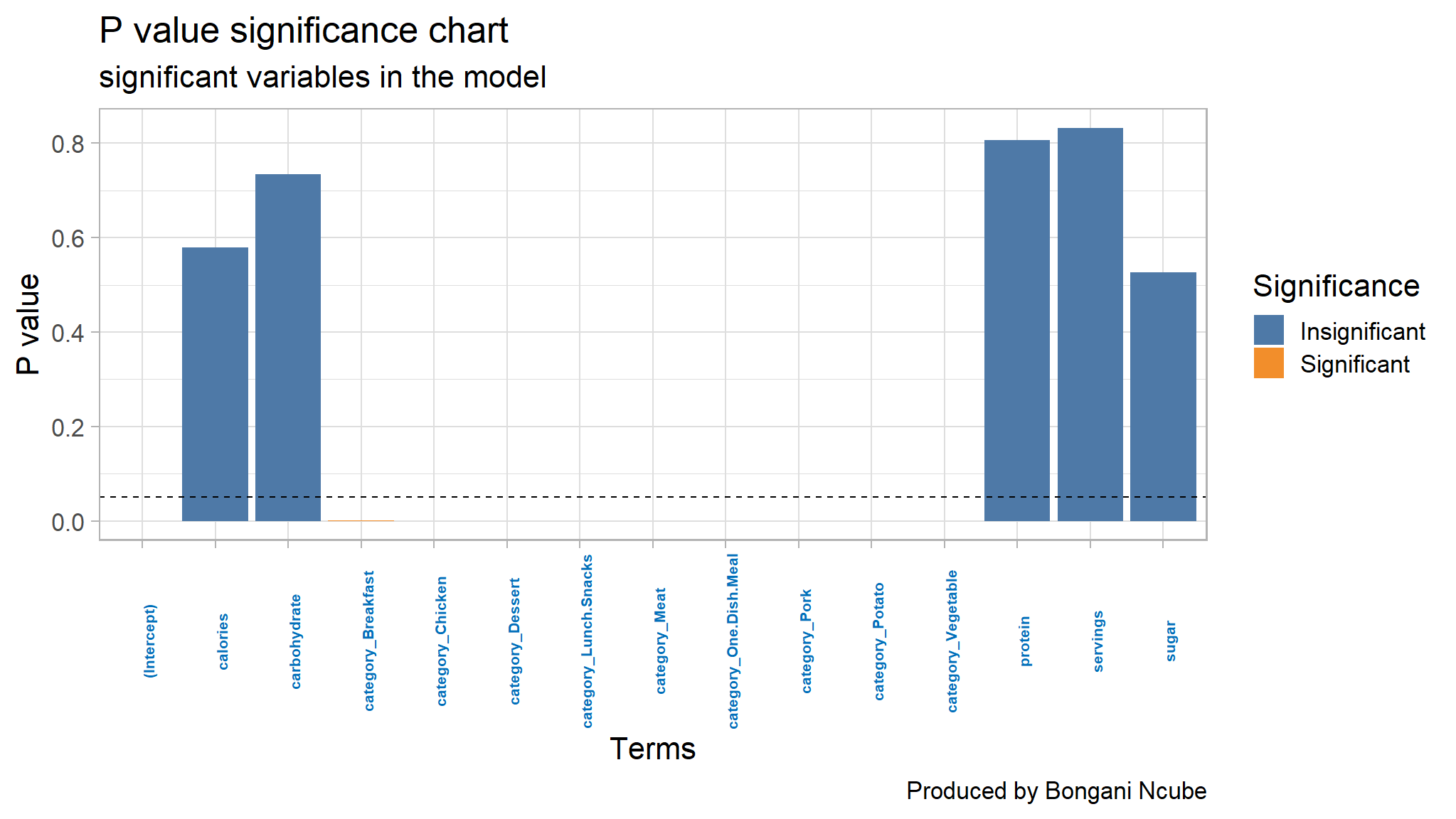
- all variables whose p value lies below the black line are
statistically significant
# Make predictions on the test set
results <- recipe_data_test|>
  select(high_traffic)|>
  bind_cols(lr_wf_fit|>
              predict(new_data = recipe_data_test))|>
  bind_cols(lr_wf_fit|>
              predict(new_data = recipe_data_test, type = "prob"))

# Print the results
results|>
  slice_head(n = 10)|> flextable()
high_traffic |
.pred_class |
.pred_0 |
.pred_1 |
|---|---|---|---|
1 |
1 |
0.05392969 |
0.9460703 |
1 |
1 |
0.05187582 |
0.9481242 |
0 |
0 |
0.55707909 |
0.4429209 |
0 |
0 |
0.53024546 |
0.4697545 |
1 |
1 |
0.24135347 |
0.7586465 |
1 |
1 |
0.20510993 |
0.7948901 |
1 |
1 |
0.23067854 |
0.7693215 |
1 |
1 |
0.05567235 |
0.9443277 |
0 |
0 |
0.69466499 |
0.3053350 |
1 |
1 |
0.33510952 |
0.6648905 |
Let’s take a look at the confusion matrix:
# Confusion matrix for prediction results
results|>
  conf_mat(truth = high_traffic, estimate = .pred_class)
#>           Truth
#> Prediction   0   1
#>          0  94  31
#>          1  26 134
# Visualize conf mat
update_geom_defaults(geom = "rect", new = list(fill = "midnightblue", alpha = 0.7))
results|>
conf_mat(high_traffic, .pred_class)|>
autoplot()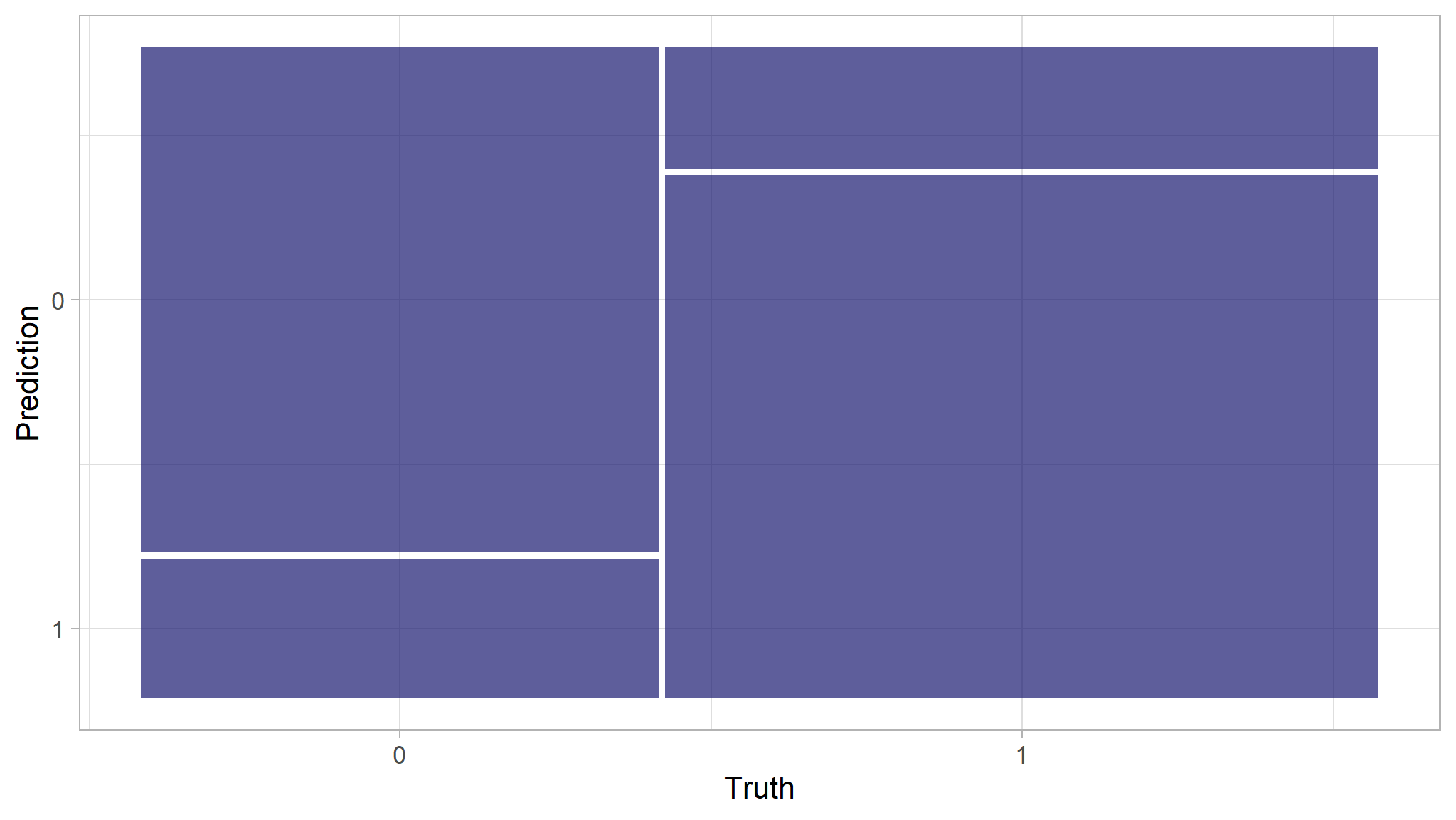
What about our other metrics such as ppv, sensitivity etc?
eval_metrics <- metric_set(ppv, recall, accuracy, f_meas)
# Evaluate other desired metrics
eval_metrics(data = results, truth = high_traffic, estimate = .pred_class)|>flextable()
.metric |
.estimator |
.estimate |
|---|---|---|
ppv |
binary |
0.7520000 |
recall |
binary |
0.7833333 |
accuracy |
binary |
0.8000000 |
f_meas |
binary |
0.7673469 |
# Evaluate ROC_AUC metrics
results|>
  roc_auc(high_traffic, .pred_0)
#> # A tibble: 1 × 3
#>   .metric .estimator .estimate
#>   <chr>   <chr>          <dbl>
#> 1 roc_auc binary         0.844

# Plot ROC_CURVE
results|>
  roc_curve(high_traffic, .pred_0)|>
  autoplot()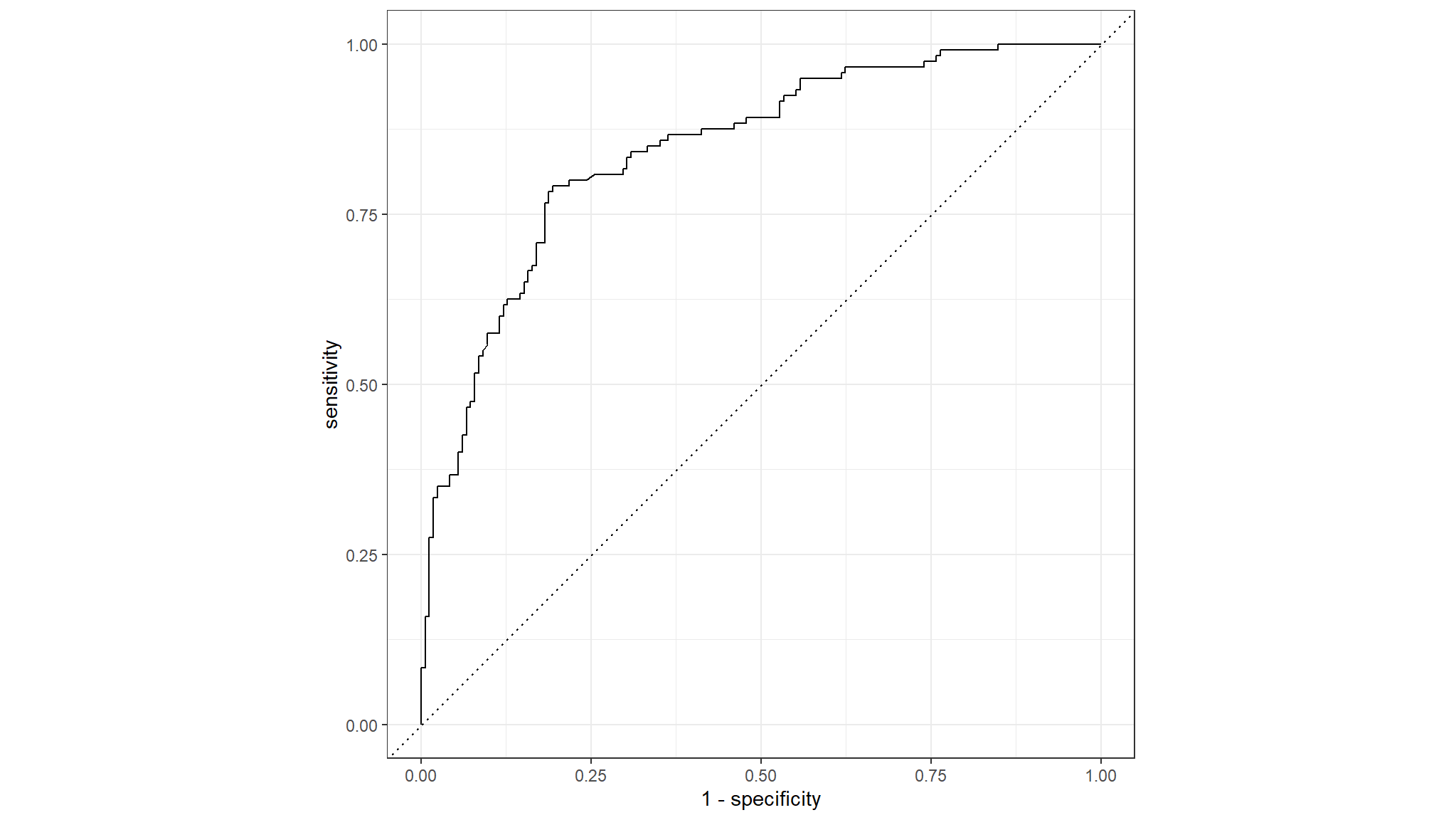
Model 2 Random forest
# Build a random forest model specification
rf_spec <- rand_forest()|>
  set_engine("ranger", importance = "impurity")|>
  set_mode("classification")

# Bundle recipe and model spec into a workflow
rf_wf <- workflow()|>
  add_recipe(recipe_data_recipe)|>
  add_model(rf_spec)

# Fit a model
rf_wf_fit <- rf_wf|>
  fit(data = recipe_data_train)

# Make predictions on test data
results <- recipe_data_test|>
  select(high_traffic)|>
  bind_cols(rf_wf_fit|>
              predict(new_data = recipe_data_test))|>
  bind_cols(rf_wf_fit|>
              predict(new_data = recipe_data_test, type = "prob"))
Model 2 : evaluation
# Confusion metrics for rf_predictions
results|>
  conf_mat(high_traffic, .pred_class)
#>           Truth
#> Prediction   0   1
#>          0  81  27
#>          1  39 138

# Confusion matrix plot
results|>
  conf_mat(high_traffic, .pred_class)|>
  autoplot()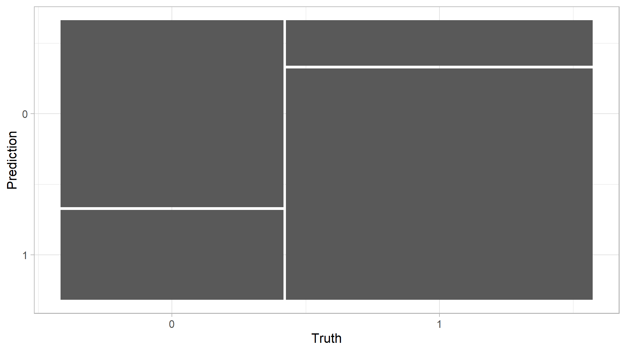
# Evaluate other intuitive classification metrics
rf_met <- results|>
  eval_metrics(truth = high_traffic, estimate = .pred_class)

# Evaluate ROC_AOC
auc <- results|>
  roc_auc(high_traffic, .pred_0)

# Plot ROC_CURVE
curve <- results|>
  roc_curve(high_traffic, .pred_0)|>
  autoplot()

# Return metrics
list(rf_met, auc, curve)
#> [[1]]
#> # A tibble: 4 × 3
#>   .metric  .estimator .estimate
#>   <chr>    <chr>          <dbl>
#> 1 ppv      binary         0.75
#> 2 recall   binary         0.675
#> 3 accuracy binary         0.768
#> 4 f_meas   binary         0.711
#>
#> [[2]]
#> # A tibble: 1 × 3
#>   .metric .estimator .estimate
#>   <chr>   <chr>          <dbl>
#> 1 roc_auc binary         0.838
#>
#> [[3]]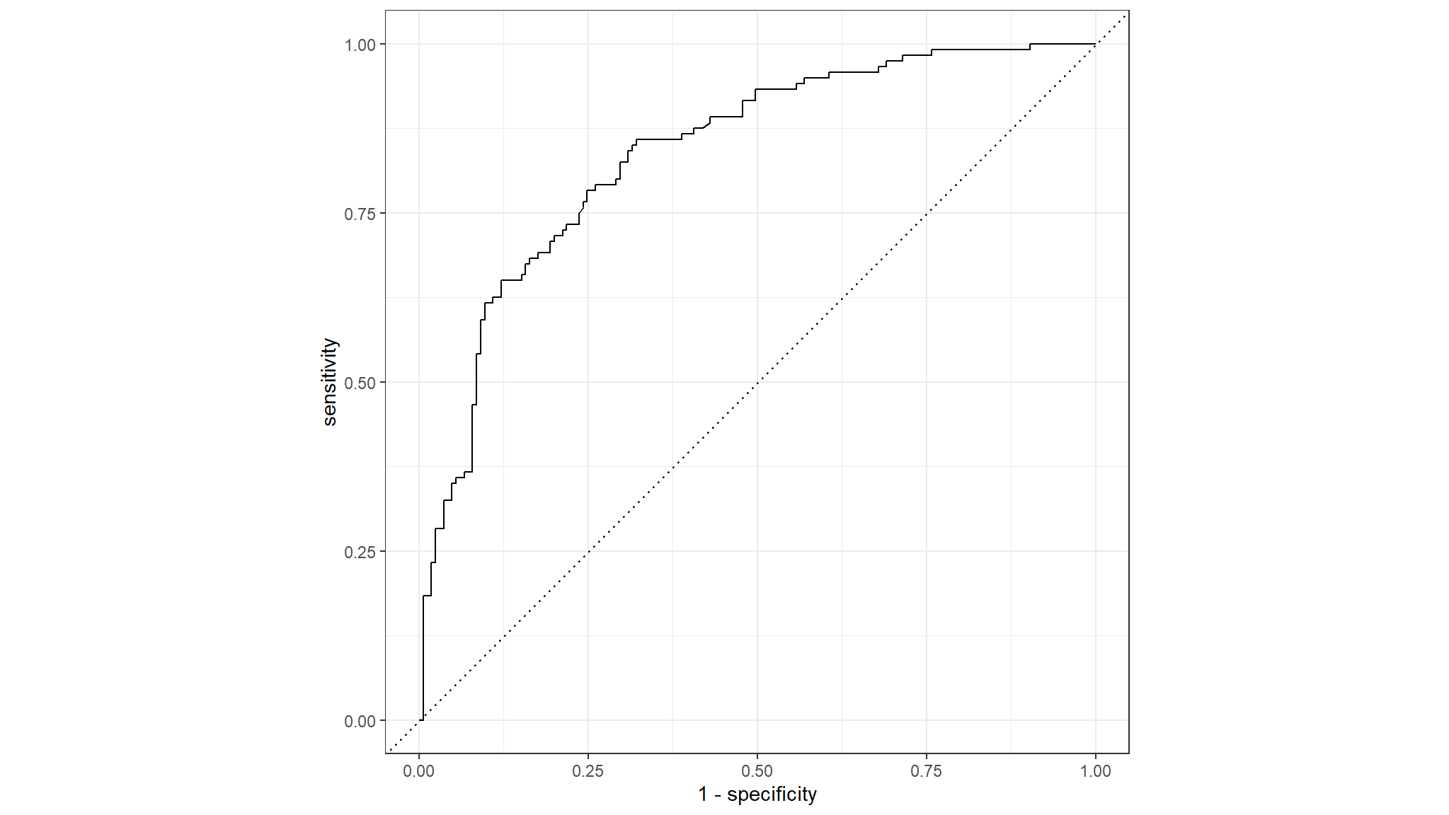
let’s make a Variable Importance Plot to see which predictor variables have the most impact in our model.
# Load vip
library(vip)

# Extract the fitted model from the workflow
rf_wf_fit|>
  extract_fit_parsnip()|>
# Make VIP plot
  vip()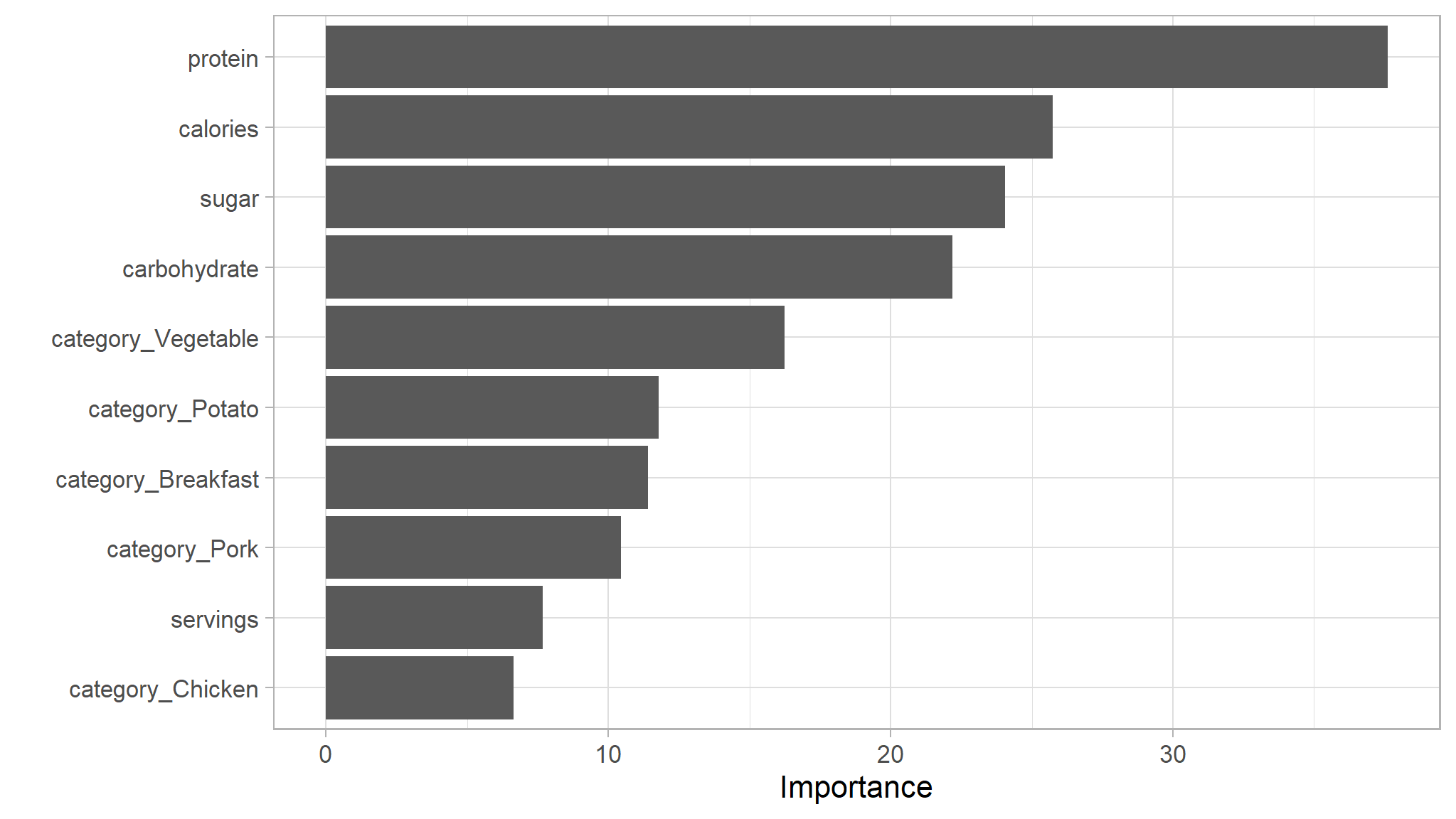
Conclusion:
Recall, Accuracy and F1 Score of High traffic by the Logistic Regression model are 0.78, 0.80, 0.76, and by Random Forest model are 0.67, 0.77, 0.71. That means the Logistic Regression model fits the features better and has less error in predicting values.
Recommendations for future actions
To help Product Manager predict the high traffic of the recipes, we can deploy this Logistic Regression Model into production. By implementing this model, about 80% of the prediction will make sure the traffic will be high. This will help Product Manager build their confidence in generating more traffic to the rest of the website.
To implement and improve the model, I will consider the following steps:
- Looking for best ways to deploy this model in terms of performance and costs. The ideal way is to deploy this machine learning model on edge devices for its convenience and security and test the model in newly hired product analysts.
- Collecting more data, e.g. time to make, cost per serving, ingredients, site duration time (how long users were at the recipe page), income links (from what sites users came to the recipe page), combinations of recipes (what recipes user visited at the same session with the current recipe).
- Feature Engineering, e.g increase number of values in category, create more meaningful features from the variables.
KPI and the performance of 2 models using KPI
The company wants to increase an accuracy of prediction of high traffic. Therefore, we would consider using accuracy of predictions which predicted high traffic as a KPI to compare 2 models again. The higher the percentage, the better the model performs. The Logistic Regression model has 80% of the accuracy whereas the accuracy of the Random Forest is lower (77%).