| spell | ui | event | logwage | married | female | age | nonwhite |
|---|---|---|---|---|---|---|---|
| 5 | 0 | 1 | 6.89568 | 1 | 0 | 41 | 0 |
| 13 | 1 | 1 | 5.28827 | 1 | 0 | 30 | 0 |
| 21 | 1 | 1 | 6.76734 | 0 | 0 | 36 | 0 |
| 3 | 1 | 1 | 5.97889 | 1 | 0 | 26 | 1 |
| 9 | 1 | 0 | 6.31536 | 0 | 0 | 22 | 0 |
| 11 | 1 | 0 | 6.85435 | 1 | 0 | 43 | 0 |
Analyzing Unemployment Duration
Be data Driven or perish
jobs
survival curves
data Driven
modeling
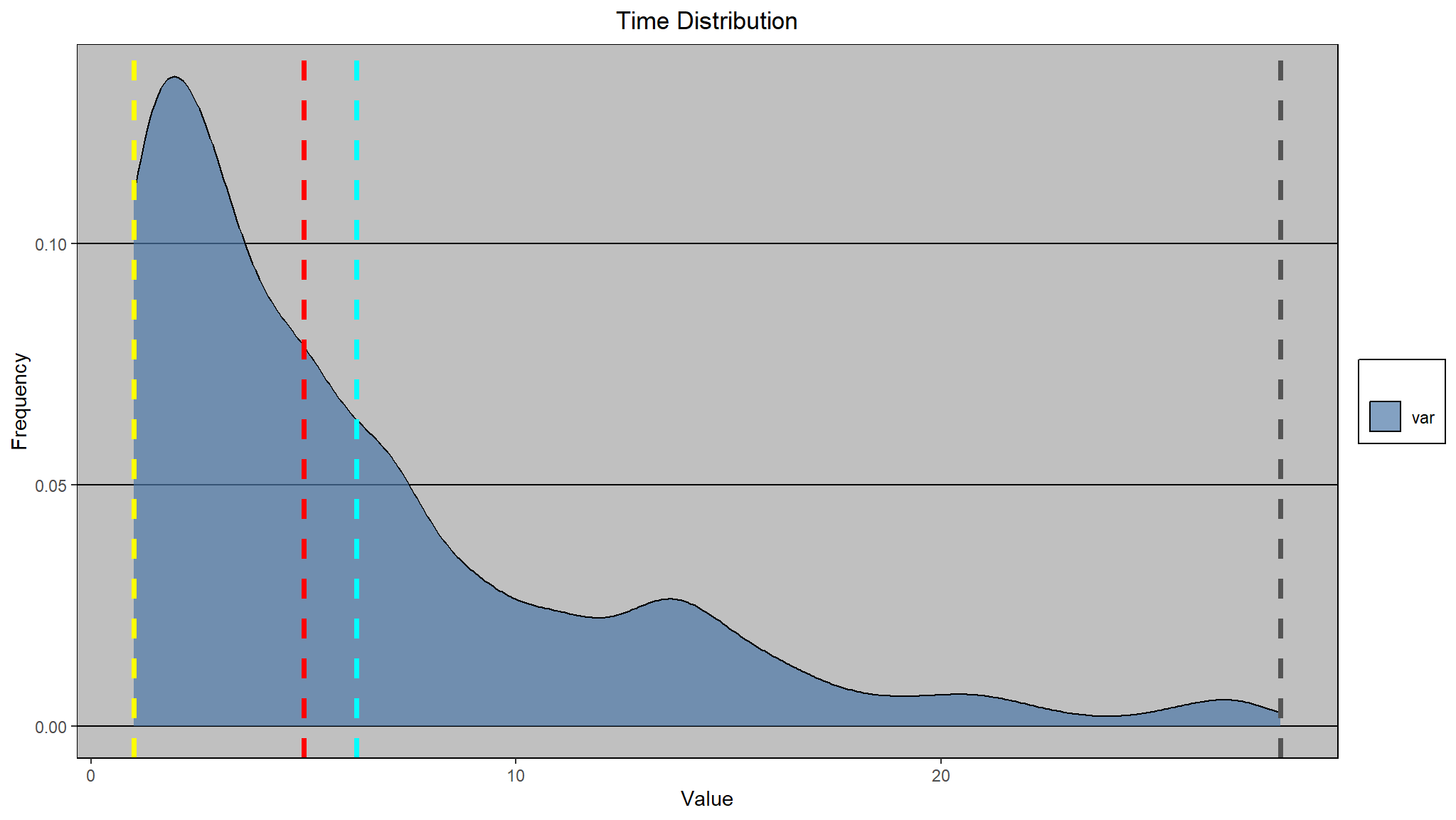
Explore survival functions for unemployment duration , we consider a cohort entering unemployment at the same time (first nonth) and we want to test if the survival rates are different for different age groups ,gender or unemployment insurance
Note
a closer look at survival analysis in unemployment
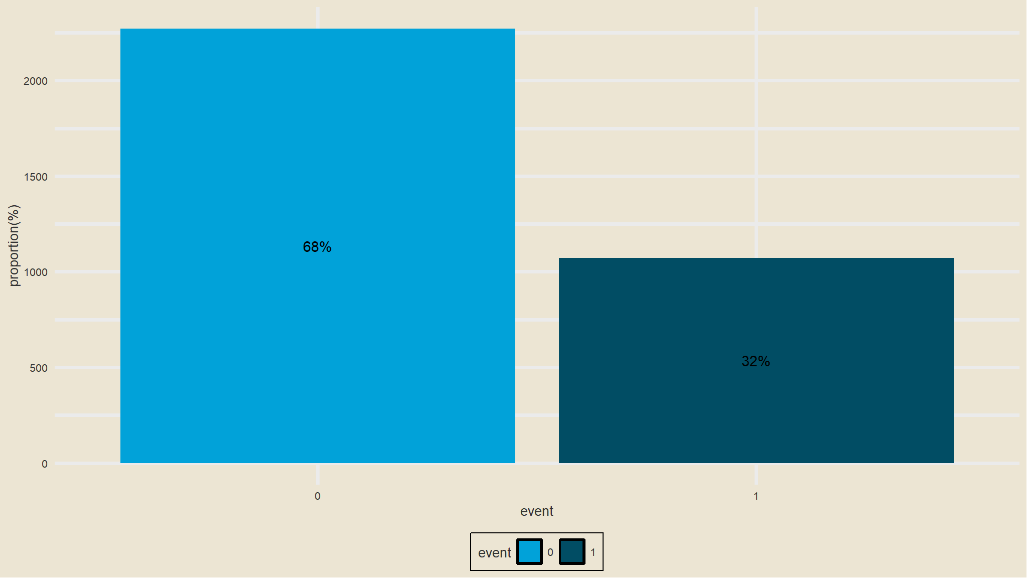
the dependent variable is made of two things
-
-
0implies a person has not found a job after9 periods(censored)
-
uistands forunemployment Insurance> the other variables are linked to that particular individual
Summary of the data at hand
Recoding the data
Explanatory Analysis
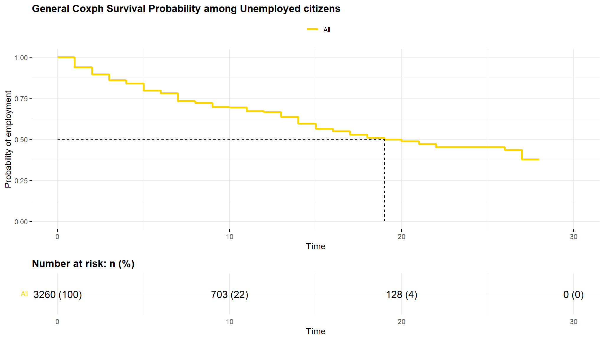
Staggered Entry situation
#> Call: survfit(formula = Surv(spell, event) ~ 1, data = out_new)
#>
#>  time n.risk n.event survival std.err lower 95% CI upper 95% CI
#>     1   3343     294    0.912 0.00490        0.903        0.922
#>     2   2803     178    0.854 0.00622        0.842        0.866
#>     3   2321     119    0.810 0.00708        0.797        0.824
#>     4   1897      56    0.786 0.00756        0.772        0.801
#>     5   1676     104    0.738 0.00847        0.721        0.754
#>     6   1339      32    0.720 0.00882        0.703        0.737
#>     7   1196      85    0.669 0.00979        0.650        0.688
#>     8    933      15    0.658 0.01001        0.639        0.678
#>     9    848      33    0.632 0.01057        0.612        0.654
#>    10    717       3    0.630 0.01064        0.609        0.651
#>    11    659      26    0.605 0.01128        0.583        0.627
#>    12    556       7    0.597 0.01150        0.575        0.620
#>    13    509      25    0.568 0.01234        0.544        0.593
#>    14    415      30    0.527 0.01353        0.501        0.554
#>    15    311      19    0.495 0.01458        0.467        0.524
#>    16    252      10    0.475 0.01527        0.446        0.506
#>    17    201       8    0.456 0.01606        0.426        0.489
#>    18    169       7    0.437 0.01691        0.405        0.472
#>    19    149       4    0.426 0.01744        0.393        0.461
#>    20    130       3    0.416 0.01794        0.382        0.452
#>    21    109       4    0.400 0.01883        0.365        0.439
#>    22     82       4    0.381 0.02029        0.343        0.423
#>    26     48       2    0.365 0.02233        0.324        0.412
#>    27     33       5    0.310 0.02964        0.257        0.374
Note
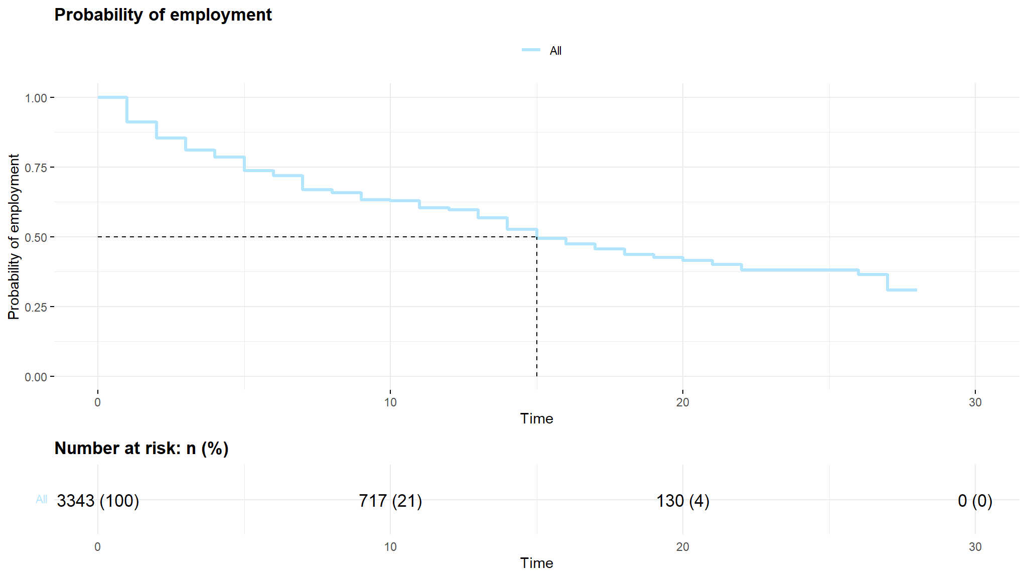
- looking at the survival curve ,note that it always starts at 1 and goes down in time
- The median survival time is
14 periods - the output table shows that the probability of
survival(= finding a job)in the first 2 months is85.4% (84.2-84.66 CI), the probability of survival gradually decreases with time in the 28 months and almost approaching zero.
Summary by gender
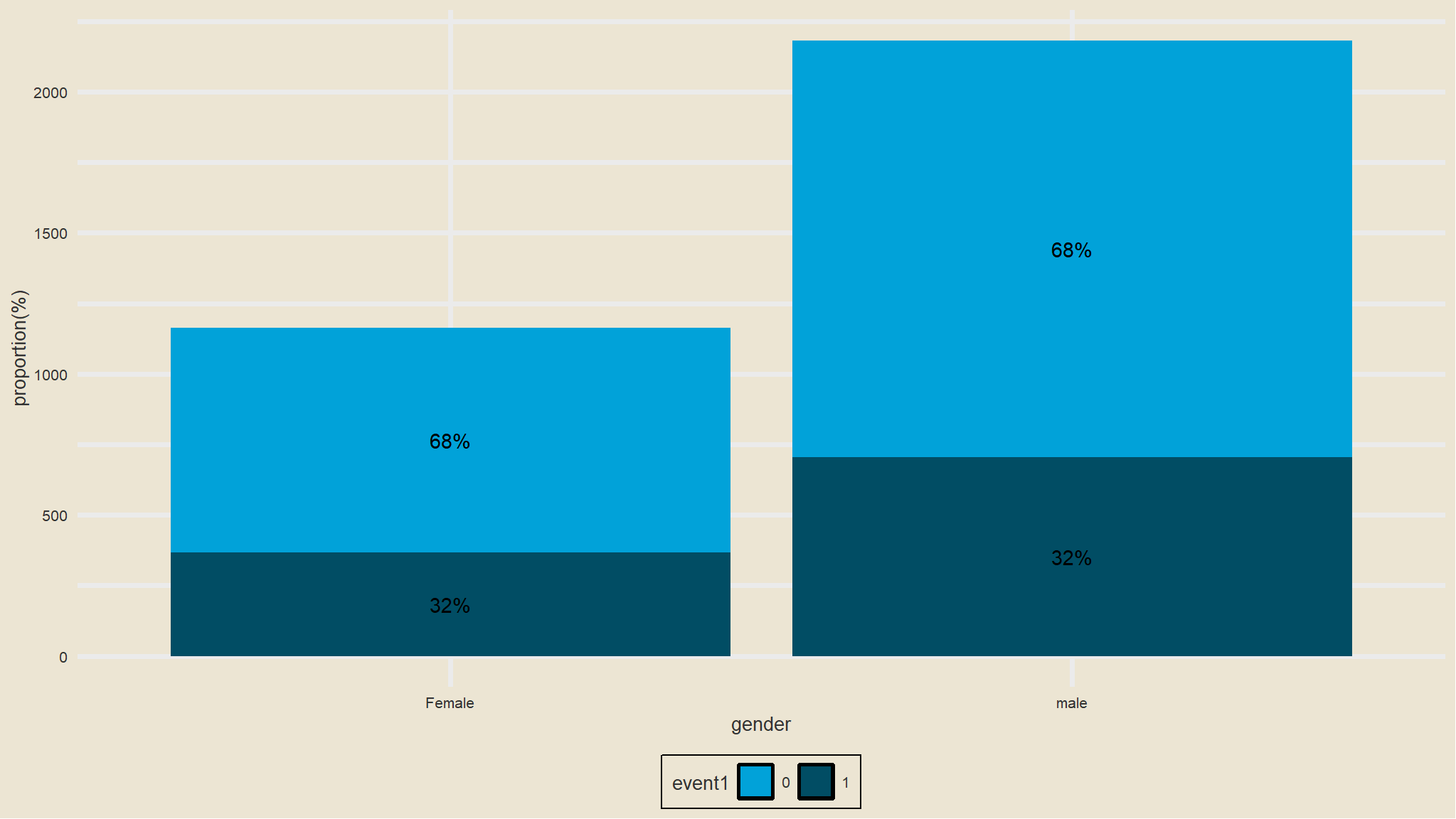
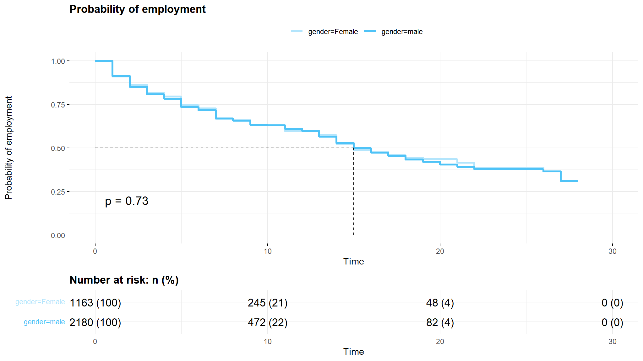
Note
- there are minor differences in the survival times (
time to get employed) between males and females
Summary by Unemployment Insurance
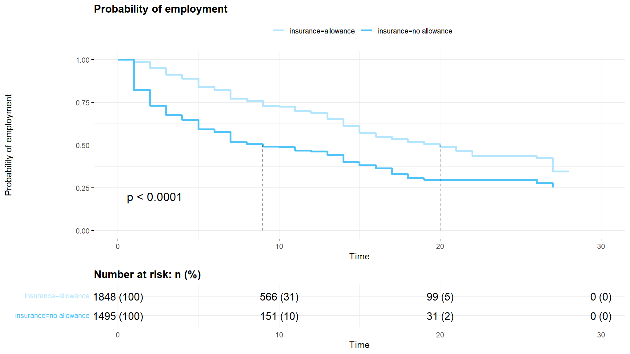
comment
- after half of the time intervals i.e (10 and 15) we see that those having unemployment benefit have about
75%survival while the other group has50%survival this means that75%of those taking allowance are still not employed after half of the time. - it can be noted from the log rank that the
survival timesbetween these groups is significantly different
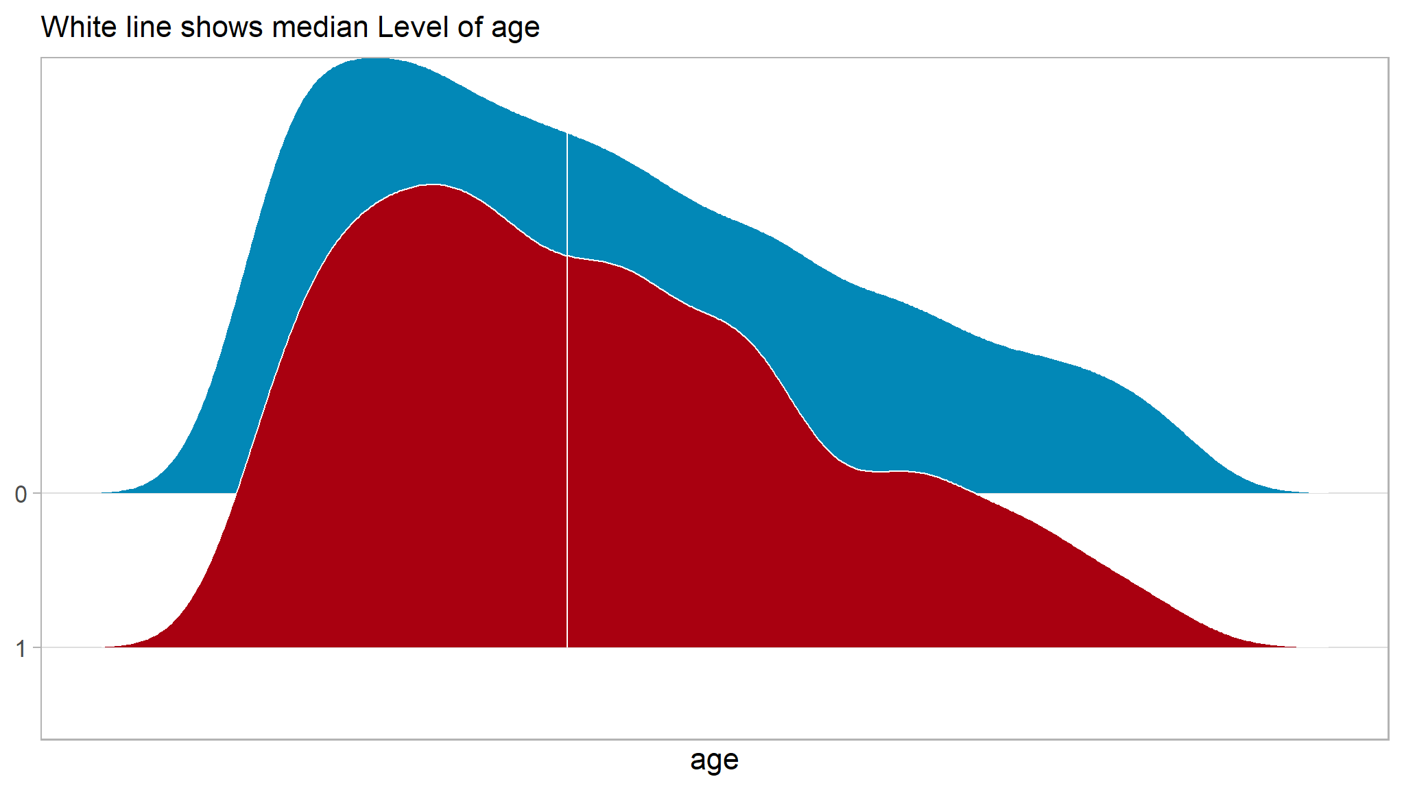
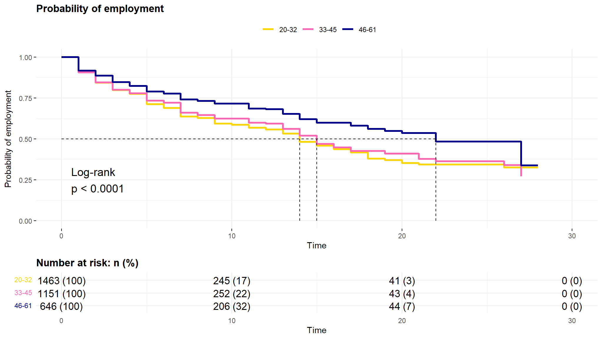
Exploring Age
- distribution of age
#> Minimum: 20.00
#> Mean: 35.44
#> Median: 34.00
#> Mode: 27.00
#> Maximum: 61.00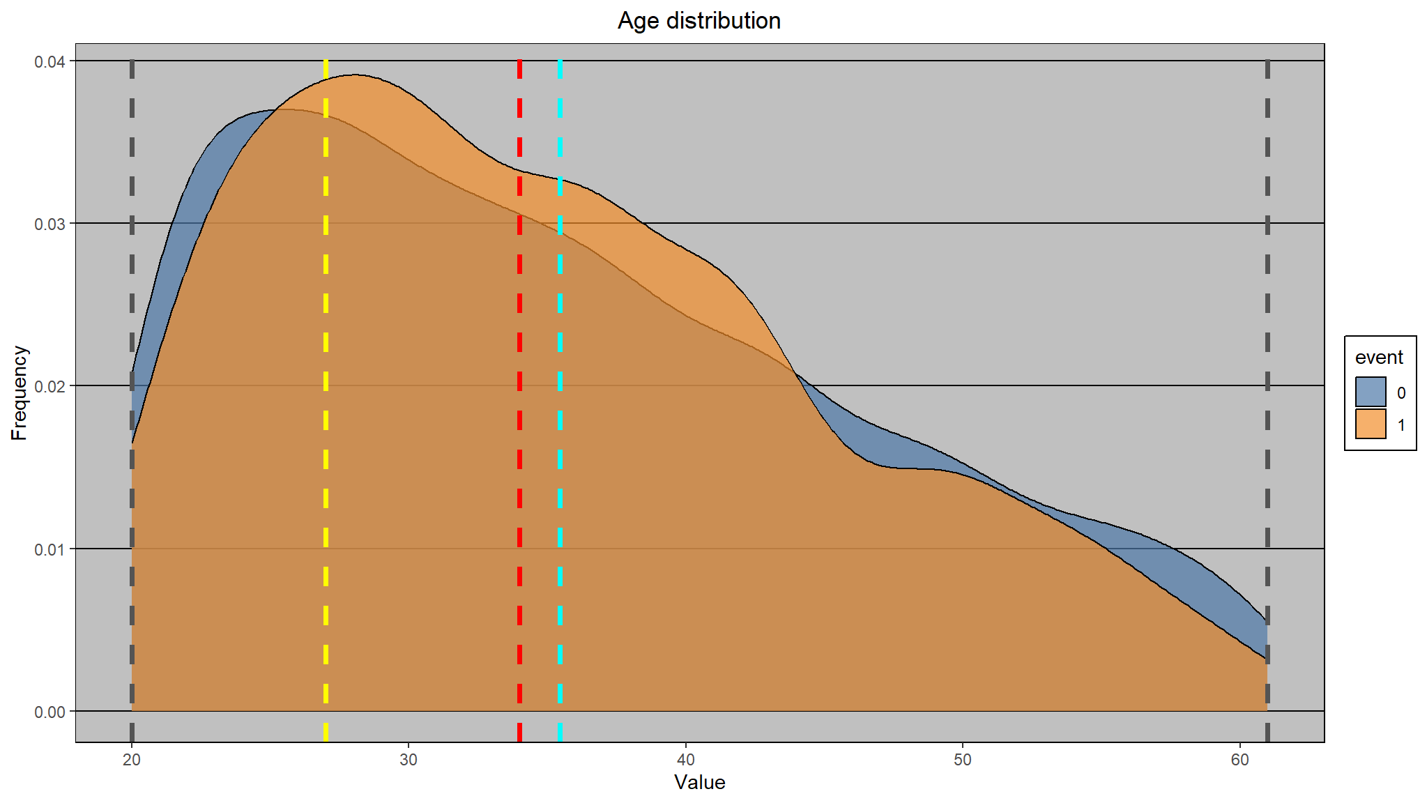
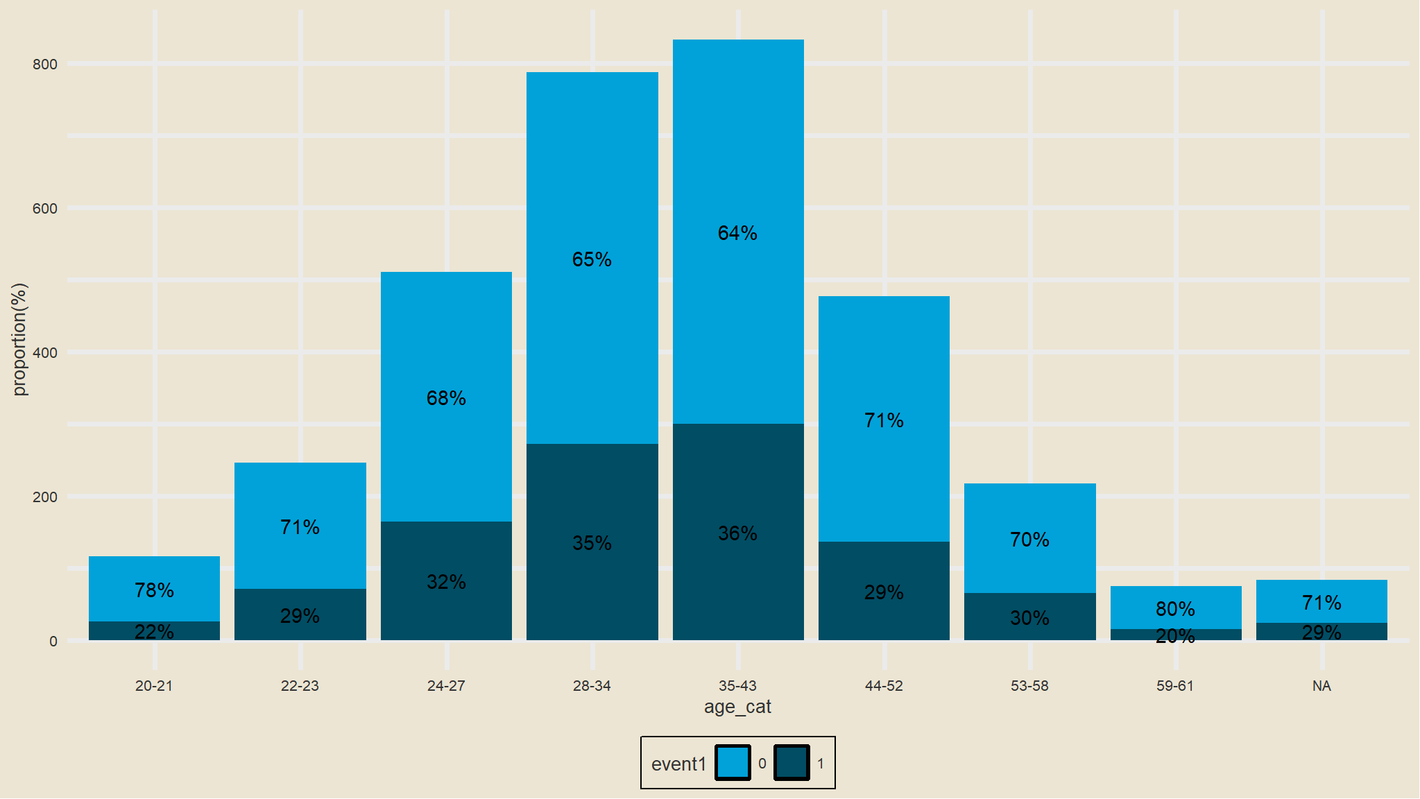
Put age into categories
- we attempt to determine weighted
(0%, 2.5%,10%,25%,50%,75%,90%,97.5%)quantiles of age and categorize the data in that order.
bins <- c(0,0.025,0.10,0.25,0.5,0.75,0.9,0.975,1)
split.Age <- wtd.quantile(out_new$age,probs=bins)
split.Age
#>    0%  2.5%   10%   25%   50%   75%   90% 97.5%  100%
#>    20    21    23    27    34    43    52    58    61
Note
the data above simply shows:
- minimum of
20 years of age - lower quartile of
27 yearsimplying that about25%are below the age of27 - median age of
34 yearsimplying that about50%are below the age of34 - upper quartile of
43 years - maximum of
61
- categorize age into the above bins
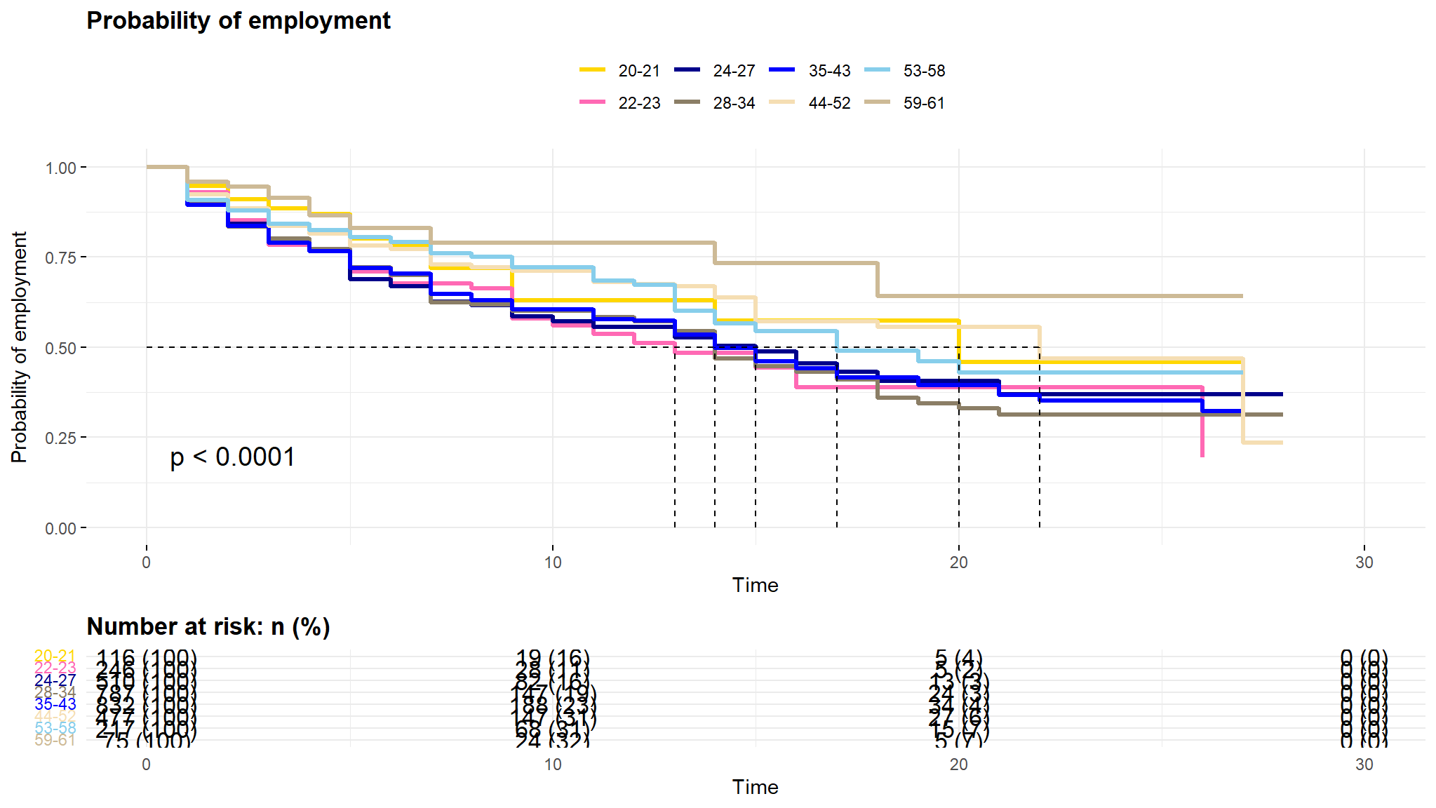
comment
- we notice a strong difference in these curves starting at
period 10and an almost inversion of them atperiod 20 - its easy and obvious to note that those in the upper
age groupsstay unemployment for a longer time implying that it is hard for the age groups44-52 and 53-61to get a job as compared to the lower age groups - those in the lower age groups get employed much faster (much easier for them to get employed)
try another binning
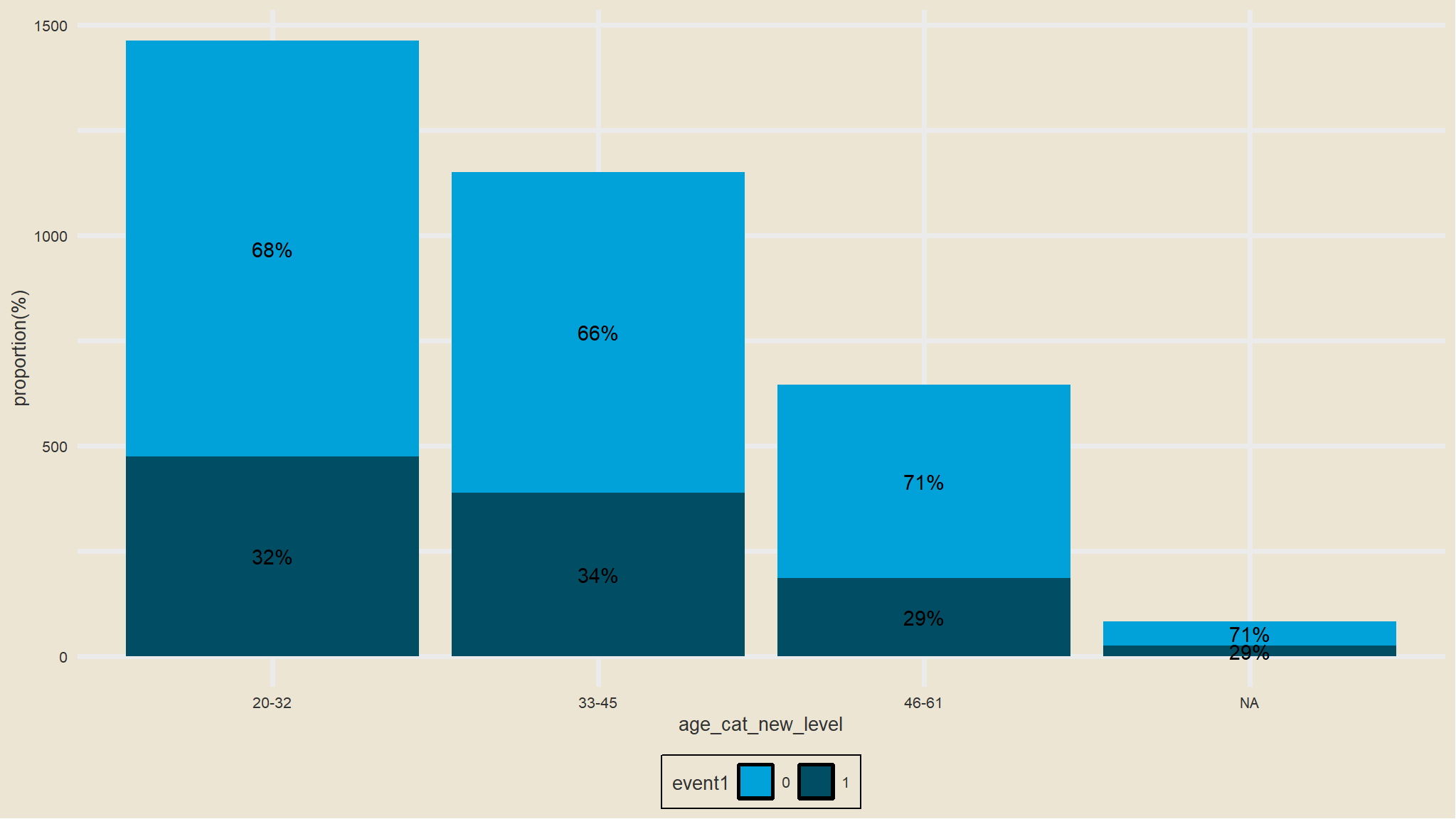
comment
- the observation is the same as from the previous age
bins
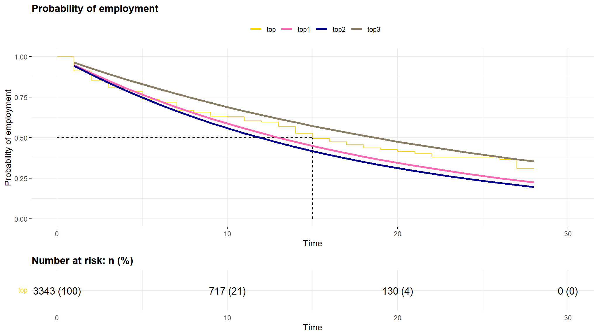
Exponential survival probability
Cox proportional Hazard
- assume
ageis not categorized
| Characteristic | HR1 | 95% CI1 | p-value |
|---|---|---|---|
| logwage | 1.69 | 1.50, 1.90 | <0.001 |
| gender | |||
| Female | — | — | |
| male | 0.86 | 0.75, 0.98 | 0.028 |
| age | 0.99 | 0.98, 1.0 | <0.001 |
| insurance | |||
| allowance | — | — | |
| no allowance | 2.79 | 2.46, 3.16 | <0.001 |
| 1 HR = Hazard Ratio, CI = Confidence Interval | |||
Comments
- holding all other covariates constant ,increase in age reduces the
hazard of employment by 0.98 - an increase in log wage increases the hazard of employment by
0.48 -
manhave a decreasedhazard of employementas compared towomen
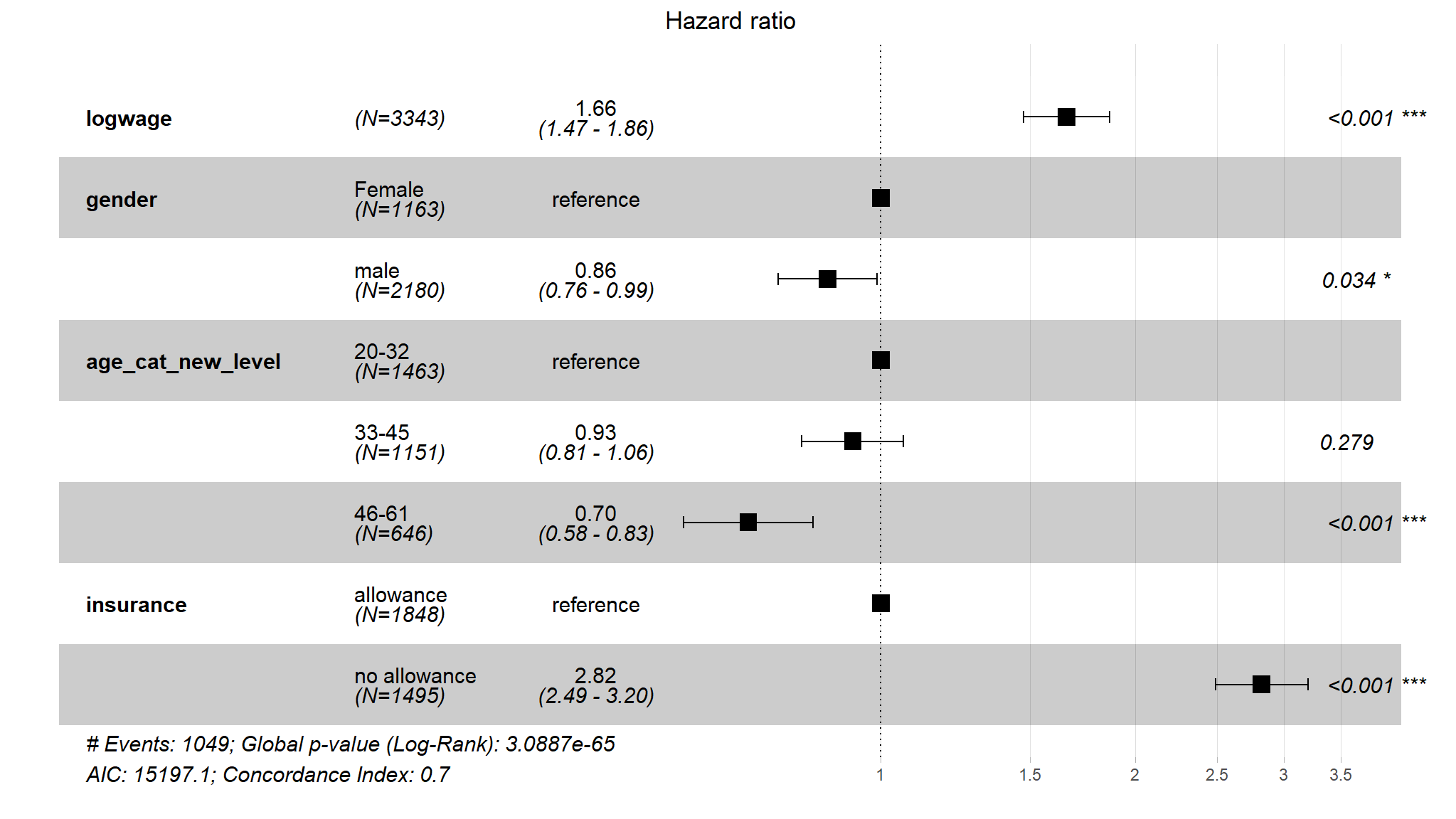
- what if age is categorised
| Characteristic | HR1 | 95% CI1 | p-value |
|---|---|---|---|
| logwage | 1.66 | 1.47, 1.86 | <0.001 |
| gender | |||
| Female | — | — | |
| male | 0.86 | 0.76, 0.99 | 0.034 |
| age_cat_new_level | |||
| 20-32 | — | — | |
| 33-45 | 0.93 | 0.81, 1.06 | 0.3 |
| 46-61 | 0.70 | 0.58, 0.83 | <0.001 |
| insurance | |||
| allowance | — | — | |
| no allowance | 2.82 | 2.49, 3.20 | <0.001 |
| 1 HR = Hazard Ratio, CI = Confidence Interval | |||
Note
- the results are almost the same , noting that the age groups
33-45and46-61have decreasedhazards of employmentas compared to the20-32age group.
which model is better
AIC(cox_m,cox_m1)
#>        df      AIC
#> cox_m   5 15197.10
#> cox_m1  4 15593.82
Note
- a model with
age categorizedperform better with a lowerAkaike Information Criterionof15451.18
Visualise the results
Conclusions
- there is no strong differences between women and men concerning their unemployment duration
- the
higher age groupshave a higher probability of remaining unemployed , i think it is harder for them to adapt to the new labor market - lastly as seen from the kaplan Meier Curve , those without
insuranceallowance have an increased hazard of employment as compared to the other group.