Modeling Claim frequency

Offsetting

generalized linear models

insurance

Published

8 February 2024

Background

Modeling claim frequency using GLMS

Offsets in Poisson models explained

In some applications, the linear predictor contains a term that requires no estimation, which is called an offset.
The offset can be viewed as a term \(\beta_jx_{ji}\) in the linear predictor for which \(\beta_j\) is known a priori.
For example, consider modelling the annual number of hospital births in various cities to facilitate resource planning. The annual number of births is discrete, so a Poisson distribution may be appropriate.
However, the expected annual number of births \(\mu_i\) ,in city i depends on the given populations \(P_i\) of the city, since cities with larger population would be expected to have more births each year, in
The number of births per unit of population, assuming a logarithmic link function, can be modelled using the systematic component \(\log(\frac{\mu}{P}) = \phi\),for the linear predictor \(\phi\).
Rearranging to model \(\mu\): \[log(\mu) = log P + \phi\]. in more mathematical terms the model without an offset is as follows

\[E(Y|X)=e^{\theta^T}x\] which simplifies to \[log(E|X)=\theta^Tx\]

while the model with an offset is given by :

\[E(Y|X)=e^{\theta^T}x*S_i\] which simplifies to \[log(E|X)=\theta^Tx+logS_i\]

The first term in the systematic component log P is completely known: nothing needs to be estimated. The term log P is called an offset. Offsets commonly appear in Poisson glms, but may appear in any glm.
The offset variable is commonly a measure of exposure. For example, the number of cases of a certain disease recorded in various mines depends on the number of workers, and also on the number of years each worker has worked in the mine.
The exposure would be the number of person-years worked in each mine, which could be incorporated into a glm as an offset. That is, a mine with many workers who have been employed for many years would be exposed to a greater likelihood of a worker contracting the disease than a mine with only a few workers who have been employed for short periods of time.

Introduction

in this analysis we have variables such as number of claims ,severity and exposure
we intend to model severity as well as number of claims per unit exposure
In this article the term exposure is a measure of what is being insured. Here an insured vehicle is an exposure. If the vehicle is insured as of July 1 for a certain year, then during that year, this would represent an exposure of 0.5 to the insurance company.

Table 1: the first six rows in our data
ID	NCLAIMS	AMOUNT	AVG	EXP	COVERAGE	FUEL	USE	FLEET	SEX	AGEPH	BM	AGEC	POWER	PC	TOWN	LONG	LAT
1	1	1618.001	1618.001	1.000	TPL	gasoline	private	N	male	50	5	12	77	1000	BRUSSEL	4.355	50.845
2	0	0.000	NA	1.000	PO	gasoline	private	N	female	64	5	3	66	1000	BRUSSEL	4.355	50.845
3	0	0.000	NA	1.000	TPL	diesel	private	N	male	60	0	10	70	1000	BRUSSEL	4.355	50.845
4	0	0.000	NA	1.000	TPL	gasoline	private	N	male	77	0	15	57	1000	BRUSSEL	4.355	50.845
5	1	155.975	155.975	0.047	TPL	gasoline	private	N	female	28	9	7	70	1000	BRUSSEL	4.355	50.845
6	0	0.000	NA	1.000	TPL	gasoline	private	N	male	26	11	12	70	1000	BRUSSEL	4.355	50.845

data Exploration

define a function to rename the variables to lower case
rename exp to exposure

out_dat <- out_new %>%
  rename_all(function(.name) {
    .name %>% 
      tolower 
  })
out_dat <-out_dat |> 
  rename(exposure = exp)

explore the dataset

what variables do we have?

names(out_dat)
#>  [1] "id"       "nclaims"  "amount"   "avg"      "exposure" "coverage"
#>  [7] "fuel"     "use"      "fleet"    "sex"      "ageph"    "bm"      
#> [13] "agec"     "power"    "pc"       "town"     "long"     "lat"

what are the data types

#>          id     nclaims      amount         avg    exposure    coverage 
#>   "integer"   "integer"   "numeric"   "numeric"   "numeric" "character" 
#>        fuel         use       fleet         sex       ageph          bm 
#> "character" "character" "character" "character"   "integer"   "integer" 
#>        agec       power          pc        town        long         lat 
#>   "integer"   "integer"   "integer" "character"   "numeric"   "numeric"

change to character to factor variables!

out_dat<-out_dat |> 
  mutate_if(is.character,as.factor)

Explanatory analysis

explore number of claims (our target variables)

plot_data<-out_dat |> 
  group_by(nclaims) %>% 
  tally() |> 
  mutate(variable="variable",
         nclaims=as.factor(nclaims)) 

g1 <- ggplot(plot_data, aes(x=nclaims,y=n,fill=variable)) + 
  theme_bw() + 
  geom_col() + 
  geom_text(aes(label=n),position=position_stack(vjust=0.5),size=2.5)+
  labs(title = "number of claims", y = "count", x ="",fill="") +
  ggthemes::scale_fill_stata() +
  theme(legend.position = "none",
        axis.text.x = element_text(face="bold", 
                                   color="black",
                                   size=8))
g1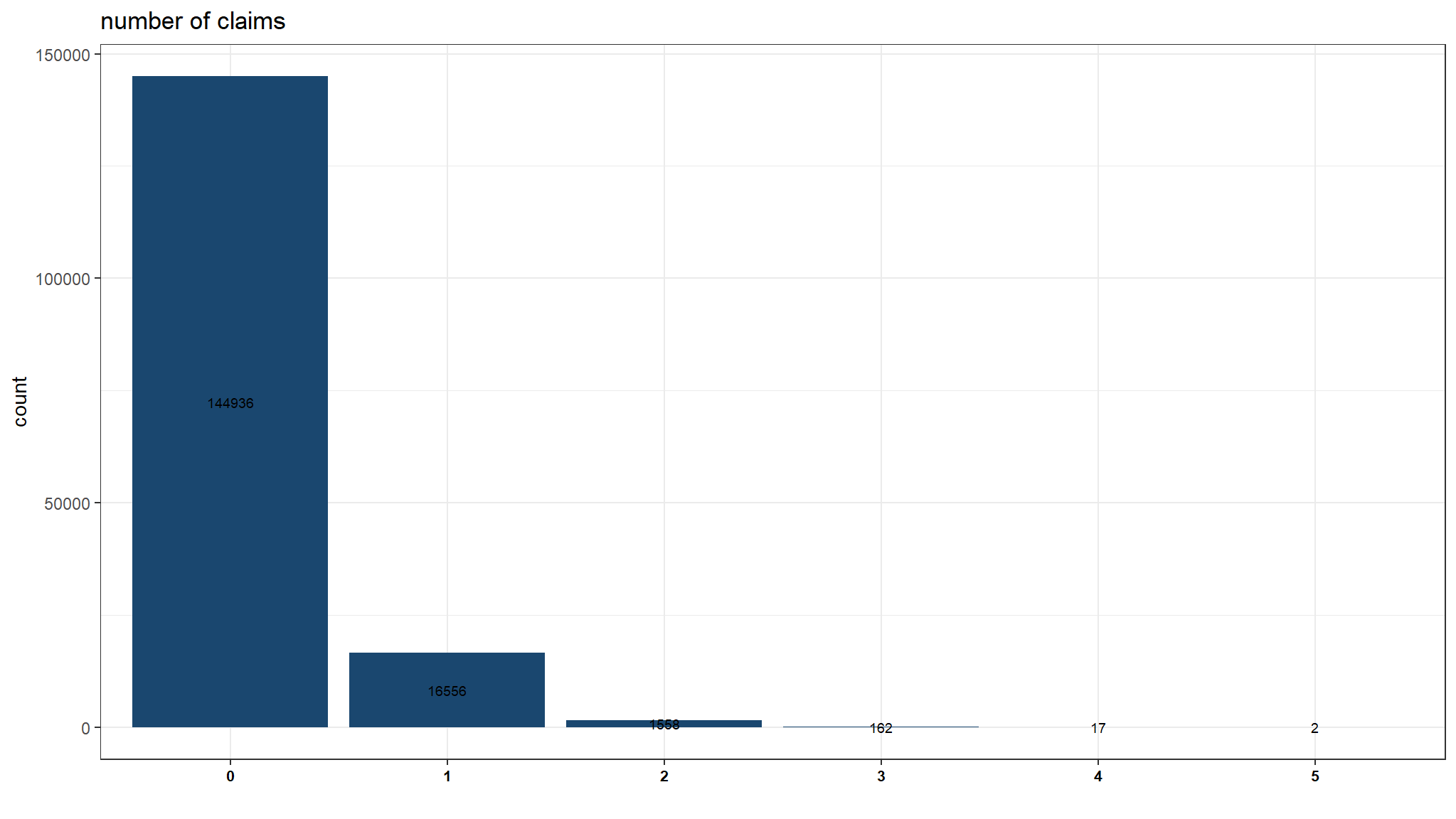

Note

number of claims is descrete(count) in nature and it can be noted that this cannot follow a normal distribution
the data is right skewed
for this reason we model using a generalized linear model (poisson to be frank)

The Poisson distribution

it specifies the probability of a discrete random variable \(Y\) and is given by:

\[f(y, \,\mu)\, =\, Pr(Y = y)\, =\, \frac{\mu^y \times e^{-\mu}}{y!}\]

\[E(Y)\, =\, Var(Y)\, =\, \mu\]

where \(\mu\) is the parameter of the Poisson distribution

The Poisson distribution is particularly relevant to model count data because it:

specifies the probability only for integer values
\(P(y<0) = 0\), hence the probability of any negative value is null
\(Var(Y) = \mu\) (the mean-variance relationship) allows for heterogeneity (e.g. when variance generally increases with the mean)

lets see if the above conditions are close

out_dat |> 
  summarise(variance=var(nclaims),
            average = mean(nclaims),
            `emperical frequency(total claims/total exposure)` = sum(nclaims) / sum(exposure),
            var =sum((nclaims -`emperical frequency(total claims/total exposure)` * exposure)^2)/sum(exposure)) |> 
  gather(key="statistic",value = "values") |> 
  knitr::kable(digits=3, "html", caption="Table 1: variance and mean are almost equal hence a poisson fits well") %>%
  kable_styling("striped", "bordered")

Table 1: variance and mean are almost equal hence a poisson fits well
statistic	values
variance	0.135
average	0.124
emperical frequency(total claims/total exposure)	0.139
var	0.152

Note

variance is almost equal to the average hence we can really see a poisson model works well here
the value var is still \(Var(Y)=E[(Y-E(Y))^2]\) were we empirically calculate the first expected value by taking exposure into account.
we then compare each realization of nclaims with its expected value i.e m*expo where m is the global empirical claim frequency

Risk classification for gender category

out_dat %>% 
  group_by(sex) %>% 
  summarise(`emperical frequency` = sum(nclaims) / sum(exposure),
            `total claims`=sum(nclaims),
            count=n()) |> 
  knitr::kable(digits=3, "html", caption="Table : summary by gender") %>%
  kable_styling("striped", "bordered")

Table : summary by gender
sex	emperical frequency	total claims	count
female	0.148	5634	43175
male	0.136	14602	120056

Note

both males and females have almost the same average emperical frequency
There were many more claims by men, although there were more men in the data. The simplest approach to analyzing these data would be to do a two-sample comparison using the poisson.test() function . It requires the counts for one or two groups.

For our application, the hypotheses to compare the two sexes are:

\[\begin{align} H_0&: \lambda_m = \lambda_f \notag \\ H_a&: \lambda_m \ne \lambda_f \notag \end{align}\]

poisson.test(c(120056   , 43175), T = 3)

#> 
#>  Comparison of Poisson rates
#> 
#> data:  c(120056, 43175) time base: 3
#> count1 = 120056, expected count1 = 81616, p-value < 2.2e-16
#> alternative hypothesis: true rate ratio is not equal to 1
#> 95 percent confidence interval:
#>  2.750243 2.811500
#> sample estimates:
#> rate ratio 
#>   2.780683

Note

The function reports a p-value as well as a confidence interval for the ratio of the claim rates. The results indicate that the observed difference is greater than the experiential noise and favors \(H_a\).

Relative frequency of claims

plot_data<-out_dat |> 
  group_by(nclaims,sex) |> 
  tally() |> 
  mutate(pct = n/sum(n)*100,
         lbl = sprintf("%.1f%%", pct)) |> 
  mutate(variable="variable",
         nclaims=as.factor(nclaims)) 

g2 <- ggplot(plot_data, aes(x=nclaims,y=n,fill=sex)) + 
  theme_bw() + 
  geom_col() + 
  geom_text(aes(label=lbl),position=position_stack(vjust=0.5),size=2.5,)+
  labs(title = "number of claims", y = "frequency(%)", x ="",fill="sex") +
  tvthemes::scale_fill_kimPossible() +
  theme(legend.position = c(0.5, 0.5),
        axis.text.x = element_text(face="bold", 
                                   color="black",
                                   size=8))
g2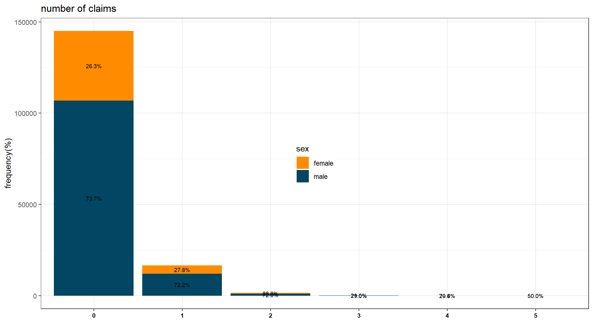

Further exploration

col <- ncube
fill <- ncube
ylab <- "Relative frequency"

# wrapper functions
ggplot.bar <- function(DT, variable, xlab){
  ggplot(data = DT, aes(as.factor(variable))) + 
  theme_bw() + 
  geom_bar(aes(y = (..count..)/sum(..count..)), 
           col = col, 
           fill = fill, 
           alpha = 0.5) + 
  labs(x = xlab, y = ylab)
}

correlation

CALIBRATING A simple GLM

like we said before , we need to include the exposure variable being offsetted hence we define offset=log(exposure)

Trivial model (null model)

freq_glm_null <- glm(nclaims ~ 1, offset = log(exposure), 
                  family = poisson(link = "log"), 
                  data = out_dat)

#> 
#> Call:
#> glm(formula = nclaims ~ 1, family = poisson(link = "log"), data = out_dat, 
#>     offset = log(exposure))
#> 
#> Coefficients:
#>             Estimate Std. Error z value Pr(>|z|)    
#> (Intercept) -1.97087    0.00703  -280.4   <2e-16 ***
#> ---
#> Signif. codes:  0 '***' 0.001 '**' 0.01 '*' 0.05 '.' 0.1 ' ' 1
#> 
#> (Dispersion parameter for poisson family taken to be 1)
#> 
#>     Null deviance: 89944  on 163230  degrees of freedom
#> Residual deviance: 89944  on 163230  degrees of freedom
#> AIC: 127678
#> 
#> Number of Fisher Scoring iterations: 6

a model with sex variable

options(scipen = 999)
freq_glm_1 <- glm(nclaims ~ sex, offset = log(exposure), 
                  family = poisson(link = "log"), 
                  data = out_dat)

#> 
#> Call:
#> glm(formula = nclaims ~ sex, family = poisson(link = "log"), 
#>     data = out_dat, offset = log(exposure))
#> 
#> Coefficients:
#>             Estimate Std. Error  z value             Pr(>|z|)    
#> (Intercept) -1.90763    0.01332 -143.186 < 0.0000000000000002 ***
#> sexmale     -0.08662    0.01568   -5.523         0.0000000333 ***
#> ---
#> Signif. codes:  0 '***' 0.001 '**' 0.01 '*' 0.05 '.' 0.1 ' ' 1
#> 
#> (Dispersion parameter for poisson family taken to be 1)
#> 
#>     Null deviance: 89944  on 163230  degrees of freedom
#> Residual deviance: 89914  on 163229  degrees of freedom
#> AIC: 127650
#> 
#> Number of Fisher Scoring iterations: 6

what do we have

generally the output suggests a model such as the following!

\[x'\beta =log(exposure)+\beta_0+\beta_1I(male)\] which when put otherwise simplifies to \[E(Y)=exposure*e^{(\beta_0+\beta_1I(male))}\]

we can also implement the same constraint using the function weights=exposure
this should literally give the same results from the previous one with offset alone.


freq_glm_sex <- glm(nclaims/exposure ~ sex, weights  = exposure, data = out_dat, family = poisson(link = "log"))

#> 
#> Call:
#> glm(formula = nclaims/exposure ~ sex, family = poisson(link = "log"), 
#>     data = out_dat, weights = exposure)
#> 
#> Coefficients:
#>             Estimate Std. Error  z value             Pr(>|z|)    
#> (Intercept) -1.90763    0.01332 -143.186 < 0.0000000000000002 ***
#> sexmale     -0.08662    0.01568   -5.523         0.0000000333 ***
#> ---
#> Signif. codes:  0 '***' 0.001 '**' 0.01 '*' 0.05 '.' 0.1 ' ' 1
#> 
#> (Dispersion parameter for poisson family taken to be 1)
#> 
#>     Null deviance: 89944  on 163230  degrees of freedom
#> Residual deviance: 89914  on 163229  degrees of freedom
#> AIC: Inf
#> 
#> Number of Fisher Scoring iterations: 6

another interesting way is to use the tidymodels , took me loads of searching to come to this
you literally need an additional package called offsetreg then follow the following steps
step 1 : define an offset variable by taking the logarithm

out_dat$offset<-log(out_dat$exposure)

step 2: now define a parsnip object using poisson_reg_offset()

glm_off<-poisson_reg_offset() |> 
  set_engine("glm_offset",offset_col="offset") |> #this would have been offset=log(exposure)
  fit(nclaims ~ sex,data=out_dat)

glm_off |> 
  pluck("fit") |> 
  summary()

#> 
#> Call:
#> stats::glm(formula = formula, family = family, data = data, offset = offset)
#> 
#> Coefficients:
#>             Estimate Std. Error  z value             Pr(>|z|)    
#> (Intercept) -1.90763    0.01332 -143.186 < 0.0000000000000002 ***
#> sexmale     -0.08662    0.01568   -5.523         0.0000000333 ***
#> ---
#> Signif. codes:  0 '***' 0.001 '**' 0.01 '*' 0.05 '.' 0.1 ' ' 1
#> 
#> (Dispersion parameter for poisson family taken to be 1)
#> 
#>     Null deviance: 89944  on 163230  degrees of freedom
#> Residual deviance: 89914  on 163229  degrees of freedom
#> AIC: 127650
#> 
#> Number of Fisher Scoring iterations: 6

Tip

If \(\beta_j = 0\) then \(exp(\beta_j) = 1\) and \(\mu\) is not related to \(x_j\). If \(\beta_j > 0\) then \(\mu\) increases if \(x_j\) increases; if \(\beta_j < 0\) then \(\mu\) decreases if \(x_j\) increases.

lets tidy this a bit

Characteristic	IRR¹	95% CI¹	p-value
sex
female	—	—
male	0.92	0.89, 0.95	<0.001
¹ IRR = Incidence Rate Ratio, CI = Confidence Interval

Note

This shows that the impact of each explanatory variable is multiplicative. being male decreases \(\mu\) by factor of exp( \(\beta_\text{sexMale}=0.92\) ) as compared to being female.

Q-square test on drop in deviance

anova(freq_glm_null,freq_glm_1,test="Chisq")
#> Analysis of Deviance Table
#> 
#> Model 1: nclaims ~ 1
#> Model 2: nclaims ~ sex
#>   Resid. Df Resid. Dev Df Deviance      Pr(>Chi)    
#> 1    163230      89944                              
#> 2    163229      89914  1   30.109 0.00000004085 ***
#> ---
#> Signif. codes:  0 '***' 0.001 '**' 0.01 '*' 0.05 '.' 0.1 ' ' 1

Note

H0 rejected in favor of more complex model H1
a model with sex performs better than an empty (null) model

attempt an `LRT` test

anova(freq_glm_null,freq_glm_1,test="LRT")
#> Analysis of Deviance Table
#> 
#> Model 1: nclaims ~ 1
#> Model 2: nclaims ~ sex
#>   Resid. Df Resid. Dev Df Deviance      Pr(>Chi)    
#> 1    163230      89944                              
#> 2    163229      89914  1   30.109 0.00000004085 ***
#> ---
#> Signif. codes:  0 '***' 0.001 '**' 0.01 '*' 0.05 '.' 0.1 ' ' 1

`Emperical claim frequency` as Driver age increases

out_dat %>% 
  group_by(ageph) %>% 
  summarise(`emperical frequency` = sum(nclaims) / sum(exposure),
            total_clm=sum(nclaims)) %>% 
  ggplot(aes(x = ageph, y = `emperical frequency`)) + 
  theme_tufte() +
  geom_point(color = ncube)+
  labs(x="Driver`s Age")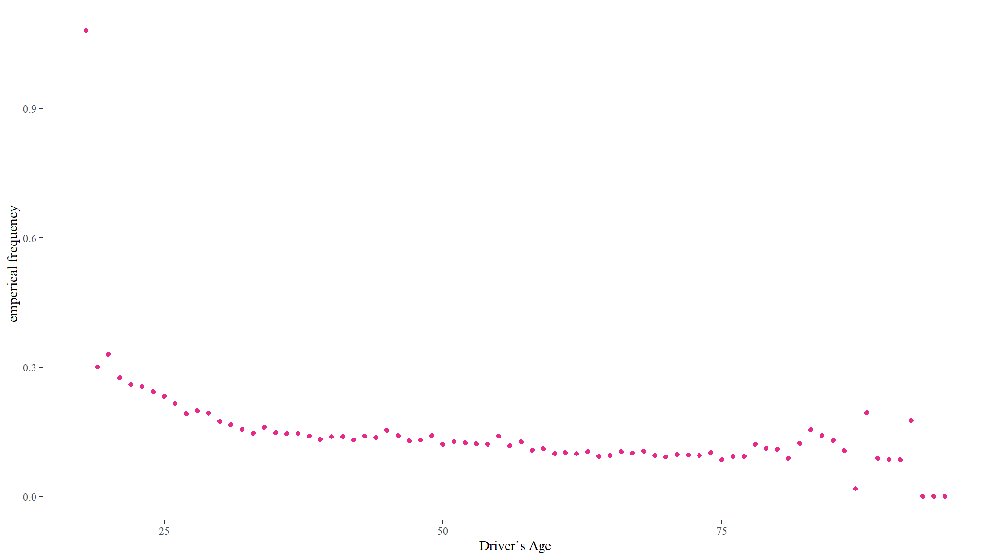

Note

the average driver’s age in the insurance portfolio is 47 years with ages ranging between 18 and 95
the plot shows that the frequency of claims is significantly different between age groups with a peak at 18 years and then declining with increasing age .

Model age and predict

freq_glm_age <- glm(nclaims ~ ageph, offset = log(exposure), data = out_dat, family = poisson(link = "log"))

#> 
#> Call:
#> glm(formula = nclaims ~ ageph, family = poisson(link = "log"), 
#>     data = out_dat, offset = log(exposure))
#> 
#> Coefficients:
#>               Estimate Std. Error z value            Pr(>|z|)    
#> (Intercept) -1.2286100  0.0229013  -53.65 <0.0000000000000002 ***
#> ageph       -0.0162582  0.0004958  -32.79 <0.0000000000000002 ***
#> ---
#> Signif. codes:  0 '***' 0.001 '**' 0.01 '*' 0.05 '.' 0.1 ' ' 1
#> 
#> (Dispersion parameter for poisson family taken to be 1)
#> 
#>     Null deviance: 89944  on 163230  degrees of freedom
#> Residual deviance: 88829  on 163229  degrees of freedom
#> AIC: 126564
#> 
#> Number of Fisher Scoring iterations: 6

tidy that up

Characteristic	IRR¹	95% CI¹	p-value
ageph	0.98	0.98, 0.98	<0.001
¹ IRR = Incidence Rate Ratio, CI = Confidence Interval

Indeed , we see that the coefficient of age was negative and the resulting value less than 1 hence an increase in age decreases \(\mu\)
at 5% level of significance , age is a significant predictor of \(\mu\)

prediction

lets do a prediction for ages in the range we already have but with an expoure of one

a <- min(out_dat$ageph):max(out_dat$ageph)

pred_glm_age <- predict(freq_glm_age, newdata = data.frame(ageph = a, exposure = 1), type = "terms", se.fit = TRUE)
b_glm_age <- pred_glm_age$fit
l_glm_age <- pred_glm_age$fit - qnorm(0.975)*pred_glm_age$se.fit
u_glm_age <- pred_glm_age$fit + qnorm(0.975)*pred_glm_age$se.fit
df <- data.frame(a, b_glm_age, l_glm_age, u_glm_age)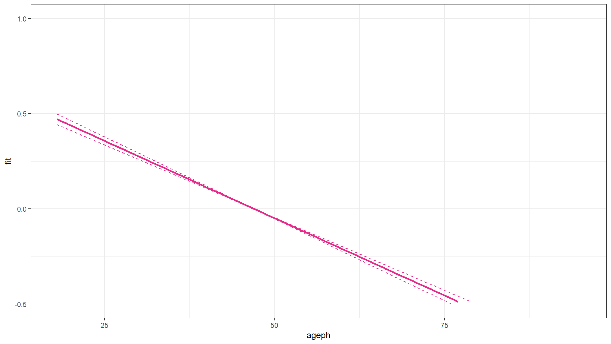

Note

expected \(\mu\) would also decrease with age .

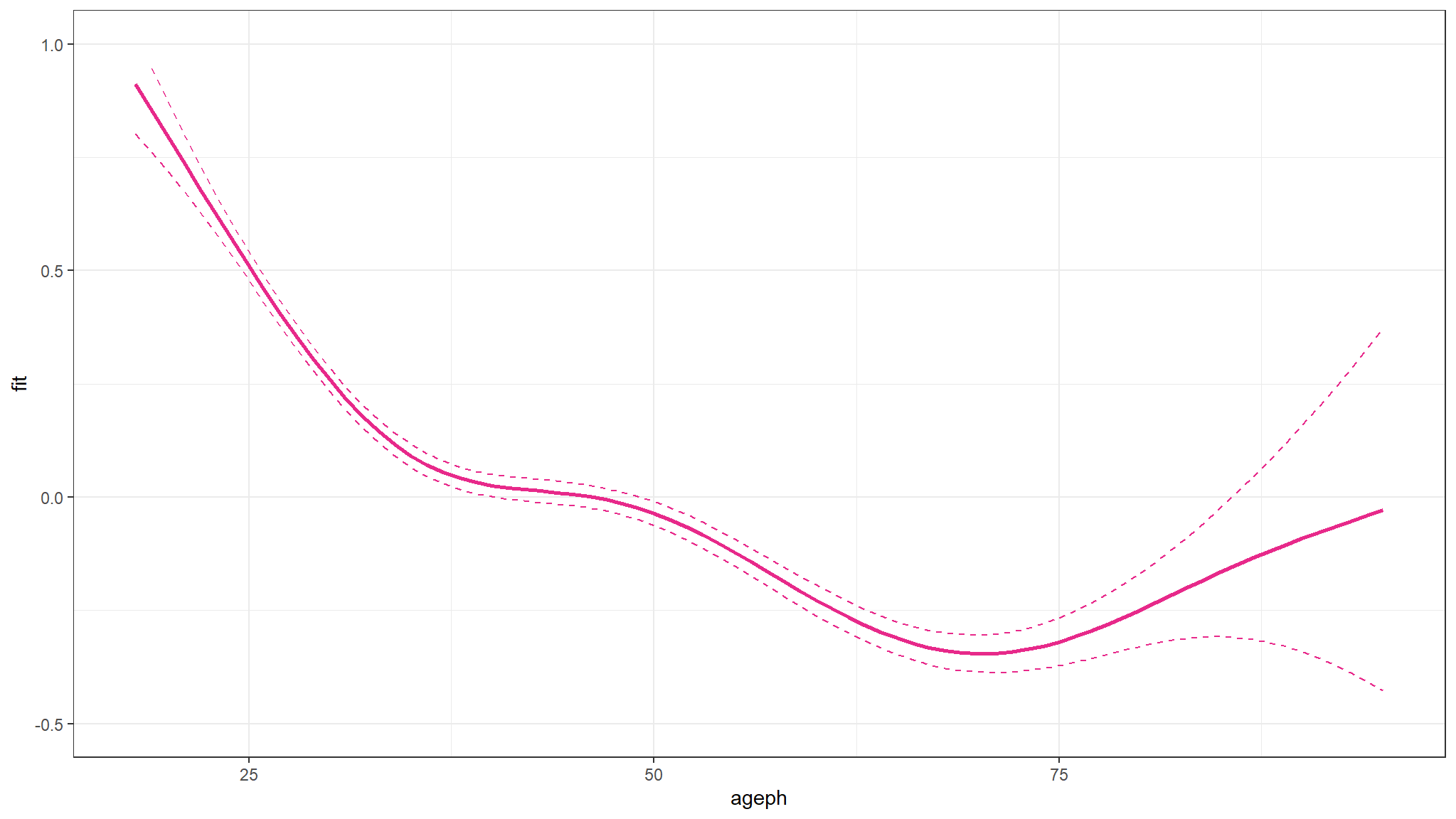
fitting a poison with a smooth function(`age variable`)!

freq_gam_age <- gam(nclaims ~ s(ageph), 
                    offset = log(exposure), 
                    data = out_dat, 
                    family = poisson(link = "log"))

#> 
#> Family: poisson 
#> Link function: log 
#> 
#> Formula:
#> nclaims ~ s(ageph)
#> 
#> Parametric coefficients:
#>              Estimate Std. Error z value            Pr(>|z|)    
#> (Intercept) -1.995268   0.007194  -277.3 <0.0000000000000002 ***
#> ---
#> Signif. codes:  0 '***' 0.001 '**' 0.01 '*' 0.05 '.' 0.1 ' ' 1
#> 
#> Approximate significance of smooth terms:
#>            edf Ref.df Chi.sq             p-value    
#> s(ageph) 5.923  6.951   1390 <0.0000000000000002 ***
#> ---
#> Signif. codes:  0 '***' 0.001 '**' 0.01 '*' 0.05 '.' 0.1 ' ' 1
#> 
#> R-sq.(adj) =  0.00853   Deviance explained = 1.47%
#> UBRE = -0.45702  Scale est. = 1         n = 163231

Note

the result shows that age is a significant smooth predictor of \(\mu\)

The figure shows that younger policyholders have a higher risk profile. The fitted GAM is lower than might be expected from the observed claim frequency for policyholders of age 19. This is because there are very few young policyholders of age 19 present in the portfolio.

prediction and prediction interval

Note

again we would expect \(\mu\) to decrease with decreasing age

Effect of putting age into categories

this allows to know exactly what happens in each category
we attempt to determine weighted (0%, 2.5%,10%,25%,50%,75%,90%,97.5%) quantiles of age and categorize the data in that order.

bins <- c(0,0.025,0.10,0.25,0.5,0.75,0.9,0.975,1)
split.Age <- wtd.quantile(out_dat$ageph,probs=bins)
split.Age
#>    0%  2.5%   10%   25%   50%   75%   90% 97.5%  100% 
#>    18    24    28    35    46    58    68    76    95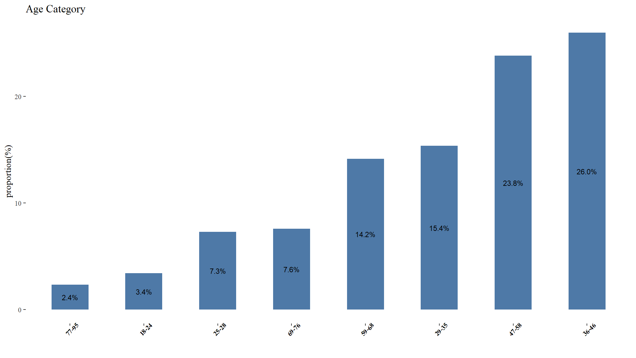

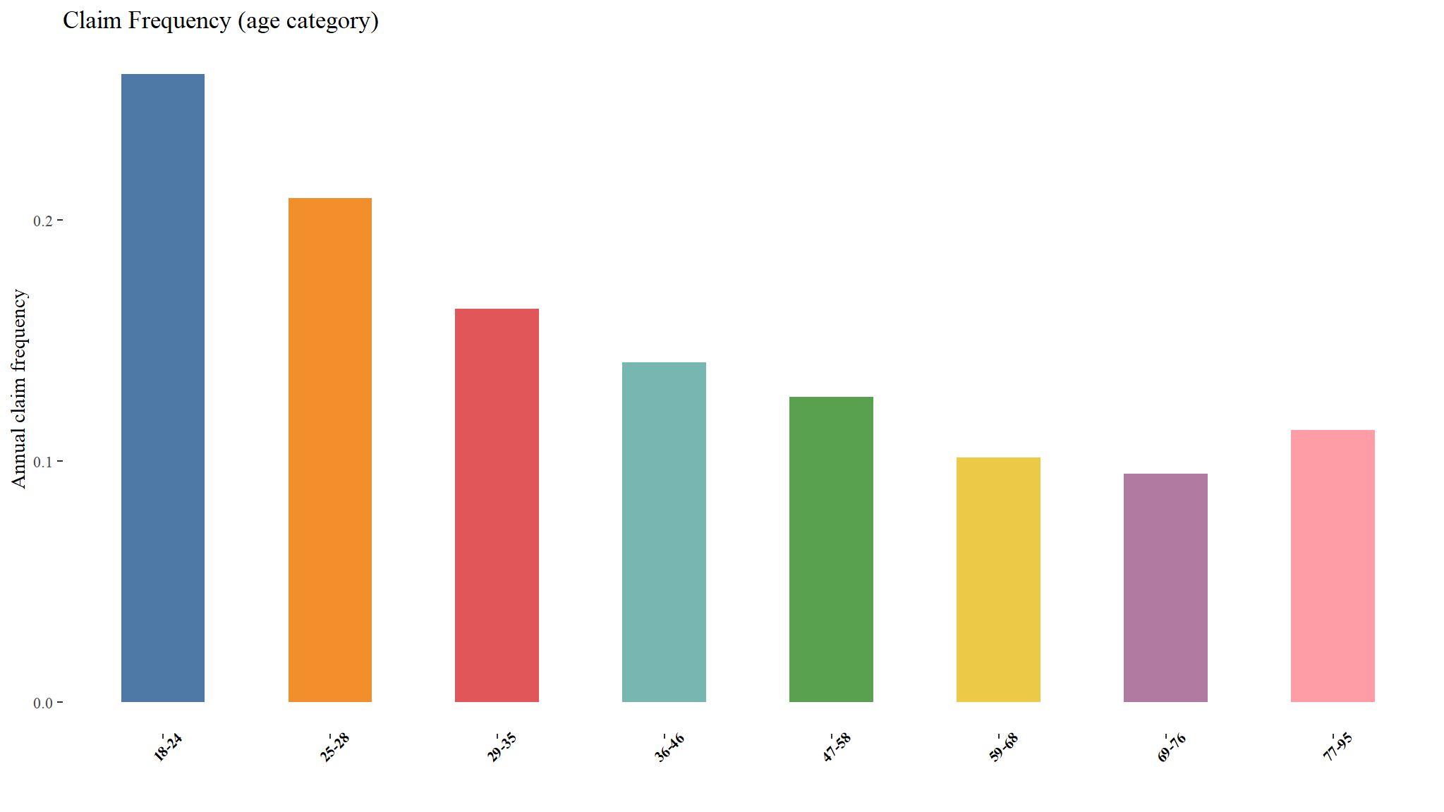
level <- c(18,24,28,35,46,58,68,76,95)
out_dat<-out_dat |> 
  mutate(age_cat=cut(ageph,level,labels=c("18-24","25-28","29-35","36-46",
                                          "47-58","59-68","69-76","77-95")),
         age_cat=if_else(is.na(age_cat),"77-95",age_cat))

Risk classification for different age classes

out_dat %>% 
  group_by(age_cat) %>% 
  summarise(`emperical frequency` = sum(nclaims) / sum(exposure),
            `total claims`=sum(nclaims),
            count=n()) |> 
  knitr::kable(digits=3, "html", caption="Table : summary by age group") %>%
  kable_styling("striped", "bordered")

Table : summary by age group
age_cat	emperical frequency	total claims	count
18-24	0.260	1231	5569
25-28	0.209	2165	11938
29-35	0.163	3521	25086
36-46	0.141	5236	42404
47-58	0.127	4429	38883
59-68	0.102	2152	23118
69-76	0.095	1101	12387
77-95	0.113	401	3846

Claim Frequency (age category)

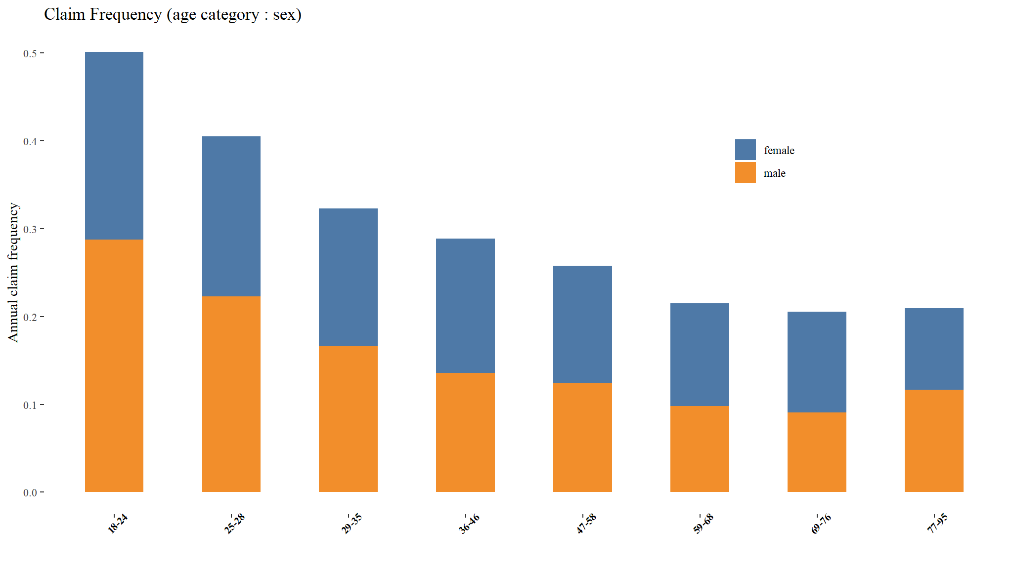
Risk classification: Possible interaction between age and sex?

out_dat %>% 
  group_by(sex,age_cat) %>% 
  summarise(`emperical frequency` = sum(nclaims) / sum(exposure),
            `total claims`=sum(nclaims),
            count=n()) |> 
  knitr::kable(digits=3, "html", caption="Table : summary by age group and sex") %>%
  kable_styling("striped", "bordered")

Table : summary by age group and sex
sex	age_cat	emperical frequency	total claims	count
female	18-24	0.214	372	2046
female	25-28	0.182	651	4133
female	29-35	0.157	1124	8325
female	36-46	0.153	1676	12556
female	47-58	0.133	1093	9244
female	59-68	0.117	448	4210
female	69-76	0.115	219	2057
female	77-95	0.093	51	604
male	18-24	0.287	859	3523
male	25-28	0.223	1514	7805
male	29-35	0.166	2397	16761
male	36-46	0.136	3560	29848
male	47-58	0.125	3336	29639
male	59-68	0.098	1704	18908
male	69-76	0.091	882	10330
male	77-95	0.116	350	3242

Claim Frequency (age category:sex)

base R has a nice way of showing this

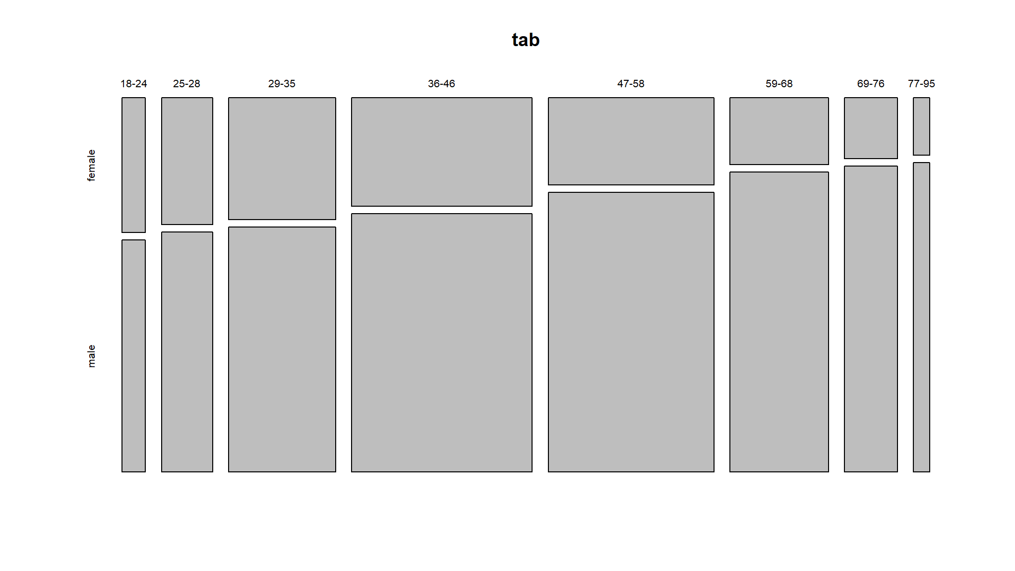
margin.table(tab,2)
#> 
#> female   male 
#>  43175 120056

We now create a model with age categorised

freq_glm_age_c <- glm(nclaims ~ age_cat, offset = log(exposure), data = out_dat, family = poisson(link = "log"))

#> 
#> Call:
#> glm(formula = nclaims ~ age_cat, family = poisson(link = "log"), 
#>     data = out_dat, offset = log(exposure))
#> 
#> Coefficients:
#>              Estimate Std. Error z value             Pr(>|z|)    
#> (Intercept)  -1.34591    0.02850 -47.222 < 0.0000000000000002 ***
#> age_cat25-28 -0.21992    0.03570  -6.161       0.000000000724 ***
#> age_cat29-35 -0.46793    0.03311 -14.132 < 0.0000000000000002 ***
#> age_cat36-46 -0.61467    0.03168 -19.405 < 0.0000000000000002 ***
#> age_cat47-58 -0.72051    0.03222 -22.362 < 0.0000000000000002 ***
#> age_cat59-68 -0.94086    0.03574 -26.328 < 0.0000000000000002 ***
#> age_cat69-76 -1.01204    0.04148 -24.398 < 0.0000000000000002 ***
#> age_cat77-95 -0.83636    0.05750 -14.546 < 0.0000000000000002 ***
#> ---
#> Signif. codes:  0 '***' 0.001 '**' 0.01 '*' 0.05 '.' 0.1 ' ' 1
#> 
#> (Dispersion parameter for poisson family taken to be 1)
#> 
#>     Null deviance: 89944  on 163230  degrees of freedom
#> Residual deviance: 88666  on 163223  degrees of freedom
#> AIC: 126414
#> 
#> Number of Fisher Scoring iterations: 6

comments

using the the simple output above we can say that ,the estimated claim frequency for each category are:

for the 25-28 category it is 0.2089145

exp(-1.34591)*exp(-0.21992)
#> [1] 0.2089145

this implies that their claim frequency is 0.802583 fold(times) higher than the claim frequency of drivers in the reference category (18-24)

exp(-0.21992)
#> [1] 0.802583

for the 29-35 category it is 0.1630269

exp(-1.34591)*exp(-0.46793)
#> [1] 0.1630269

this implies that their claim frequency is 0.6262974 fold(times) higher than the claim frequency of drivers in the reference category (18-24)

exp(-0.46793)
#> [1] 0.6262974

for the 36-46 category it is 0.1407767

exp(-1.34591)*exp(-0.61467)
#> [1] 0.1407767

this implies that their claim frequency is 0.5408193 fold(times) higher than the claim frequency of drivers in the reference category (18-24)

exp(-0.61467)
#> [1] 0.5408193

for the 47-58 category it is 0.1266383

exp(-1.34591)*exp(-0.72051)
#> [1] 0.1266383

this implies that their claim frequency is 0.4865041 fold(times) higher than the claim frequency of drivers in the reference category (18-24)

exp(-0.72051)
#> [1] 0.4865041

for the 59-68 category it is 0.1015941

exp(-1.34591)*exp(-0.94086)
#> [1] 0.1015941

this implies that their claim frequency is 0.390292 fold(times) higher than the claim frequency of drivers in the reference category (18-24)

exp(-0.94086)
#> [1] 0.390292

for the 69-76 category it is 0.09461398

exp(-1.34591)*exp(-1.01204)
#> [1] 0.09461398

this implies that their claim frequency is 0.404898 fold(times) higher than the claim frequency of drivers in the reference category (18-24)

exp(-1.01204)
#> [1] 0.3634767

for the 77-95 category it is 0.1127852

exp(-1.34591)*exp(-0.83636)
#> [1] 0.1127852

this implies that their claim frequency is 0.4332848 fold(times) higher than the claim frequency of drivers in the reference category (18-24)

exp(-0.83636)
#> [1] 0.4332848

Generally

we note that the estimated claim frequency generally decreases going to higher age categories

tidy that a bit

Characteristic	IRR¹	95% CI¹	p-value
age_cat
18-24	—	—
25-28	0.80	0.75, 0.86	<0.001
29-35	0.63	0.59, 0.67	<0.001
36-46	0.54	0.51, 0.58	<0.001
47-58	0.49	0.46, 0.52	<0.001
59-68	0.39	0.36, 0.42	<0.001
69-76	0.36	0.34, 0.39	<0.001
77-95	0.43	0.39, 0.48	<0.001
¹ IRR = Incidence Rate Ratio, CI = Confidence Interval

look at the prediction for this model

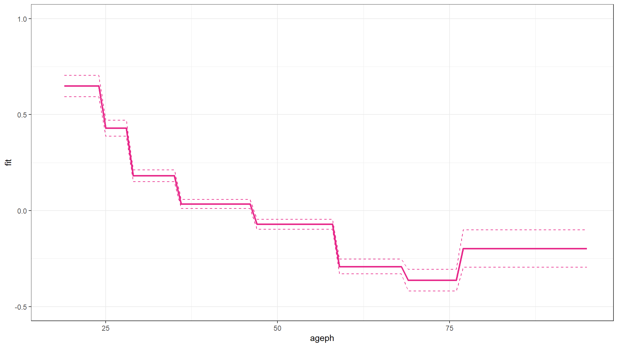
to add on

the prediction plot is for those who have an exact exposure of 1 since this is the most frequent exposure value
our prediction using the model suggests that as age increases , claim frequency decreases for individuals with an exposure value of one

try a model with age and sex

freq_glm_age_sex <- glm(nclaims ~ age_cat+sex, offset = log(exposure), data = out_dat, family = poisson(link = "log"))

#> 
#> Call:
#> glm(formula = nclaims ~ age_cat + sex, family = poisson(link = "log"), 
#>     data = out_dat, offset = log(exposure))
#> 
#> Coefficients:
#>              Estimate Std. Error z value             Pr(>|z|)    
#> (Intercept)  -1.33797    0.03019 -44.314 < 0.0000000000000002 ***
#> age_cat25-28 -0.21962    0.03570  -6.152       0.000000000765 ***
#> age_cat29-35 -0.46747    0.03312 -14.116 < 0.0000000000000002 ***
#> age_cat36-46 -0.61375    0.03170 -19.363 < 0.0000000000000002 ***
#> age_cat47-58 -0.71882    0.03229 -22.262 < 0.0000000000000002 ***
#> age_cat59-68 -0.93850    0.03586 -26.171 < 0.0000000000000002 ***
#> age_cat69-76 -1.00946    0.04161 -24.262 < 0.0000000000000002 ***
#> age_cat77-95 -0.83366    0.05760 -14.473 < 0.0000000000000002 ***
#> sexmale      -0.01261    0.01584  -0.796                0.426    
#> ---
#> Signif. codes:  0 '***' 0.001 '**' 0.01 '*' 0.05 '.' 0.1 ' ' 1
#> 
#> (Dispersion parameter for poisson family taken to be 1)
#> 
#>     Null deviance: 89944  on 163230  degrees of freedom
#> Residual deviance: 88666  on 163222  degrees of freedom
#> AIC: 126415
#> 
#> Number of Fisher Scoring iterations: 6

Characteristic	IRR¹	95% CI¹	p-value
age_cat
18-24	—	—
25-28	0.80	0.75, 0.86	<0.001
29-35	0.63	0.59, 0.67	<0.001
36-46	0.54	0.51, 0.58	<0.001
47-58	0.49	0.46, 0.52	<0.001
59-68	0.39	0.36, 0.42	<0.001
69-76	0.36	0.34, 0.40	<0.001
77-95	0.43	0.39, 0.49	<0.001
sex
female	—	—
male	0.99	0.96, 1.02	0.4
¹ IRR = Incidence Rate Ratio, CI = Confidence Interval

model building using `AIC`

freq_glm_full <- glm(nclaims ~ ageph+sex+coverage+use+fuel+fleet+pc+bm+power+agec, offset = log(exposure), data = out_dat, family = poisson(link = "log"))
MASS::stepAIC(freq_glm_full,direction="both")
#> Start:  AIC=124988.1
#> nclaims ~ ageph + sex + coverage + use + fuel + fleet + pc + 
#>     bm + power + agec
#> 
#>            Df Deviance    AIC
#> - agec      1    87233 124986
#> - sex       1    87234 124988
#> <none>           87233 124988
#> - use       1    87239 124992
#> - fleet     1    87241 124994
#> - coverage  2    87271 125022
#> - power     1    87324 125078
#> - pc        1    87350 125103
#> - fuel      1    87361 125115
#> - ageph     1    87446 125199
#> - bm        1    88464 126217
#> 
#> Step:  AIC=124986.5
#> nclaims ~ ageph + sex + coverage + use + fuel + fleet + pc + 
#>     bm + power
#> 
#>            Df Deviance    AIC
#> - sex       1    87235 124986
#> <none>           87233 124986
#> + agec      1    87233 124988
#> - use       1    87239 124991
#> - fleet     1    87241 124993
#> - coverage  2    87275 125024
#> - power     1    87329 125080
#> - pc        1    87350 125102
#> - fuel      1    87365 125116
#> - ageph     1    87449 125200
#> - bm        1    88466 126217
#> 
#> Step:  AIC=124986.1
#> nclaims ~ ageph + coverage + use + fuel + fleet + pc + bm + power
#> 
#>            Df Deviance    AIC
#> <none>           87235 124986
#> + sex       1    87233 124986
#> + agec      1    87234 124988
#> - use       1    87241 124990
#> - fleet     1    87243 124992
#> - coverage  2    87276 125023
#> - power     1    87329 125078
#> - pc        1    87353 125102
#> - fuel      1    87365 125114
#> - ageph     1    87458 125207
#> - bm        1    88474 126223
#> 
#> Call:  glm(formula = nclaims ~ ageph + coverage + use + fuel + fleet + 
#>     pc + bm + power, family = poisson(link = "log"), data = out_dat, 
#>     offset = log(exposure))
#> 
#> Coefficients:
#>  (Intercept)         ageph    coveragePO   coverageTPL       usework  
#>  -1.83493214   -0.00792846   -0.00037807    0.09498288   -0.08180670  
#> fuelgasoline        fleetY            pc            bm         power  
#>  -0.17350485   -0.11981008   -0.00002857    0.06277044    0.00365499  
#> 
#> Degrees of Freedom: 163230 Total (i.e. Null);  163221 Residual
#> Null Deviance:       89940 
#> Residual Deviance: 87230     AIC: 125000

final<-glm(formula = nclaims ~ ageph + coverage + use + fuel + fleet + 
    pc + bm + power, family = poisson(link = "log"), data = out_dat, 
    offset = log(exposure))

#> 
#> Call:
#> glm(formula = nclaims ~ ageph + coverage + use + fuel + fleet + 
#>     pc + bm + power, family = poisson(link = "log"), data = out_dat, 
#>     offset = log(exposure))
#> 
#> Coefficients:
#>                  Estimate   Std. Error z value             Pr(>|z|)    
#> (Intercept)  -1.834932140  0.043351298 -42.327 < 0.0000000000000002 ***
#> ageph        -0.007928458  0.000536976 -14.765 < 0.0000000000000002 ***
#> coveragePO   -0.000378075  0.023952053  -0.016               0.9874    
#> coverageTPL   0.094982885  0.022089619   4.300            0.0000171 ***
#> usework      -0.081806695  0.033446860  -2.446               0.0145 *  
#> fuelgasoline -0.173504852  0.015079149 -11.506 < 0.0000000000000002 ***
#> fleetY       -0.119810081  0.043512007  -2.753               0.0059 ** 
#> pc           -0.000028574  0.000002633 -10.854 < 0.0000000000000002 ***
#> bm            0.062770436  0.001729931  36.285 < 0.0000000000000002 ***
#> power         0.003654994  0.000370316   9.870 < 0.0000000000000002 ***
#> ---
#> Signif. codes:  0 '***' 0.001 '**' 0.01 '*' 0.05 '.' 0.1 ' ' 1
#> 
#> (Dispersion parameter for poisson family taken to be 1)
#> 
#>     Null deviance: 89944  on 163230  degrees of freedom
#> Residual deviance: 87235  on 163221  degrees of freedom
#> AIC: 124986
#> 
#> Number of Fisher Scoring iterations: 6

Characteristic	IRR¹	95% CI¹	p-value
ageph	0.99	0.99, 0.99	<0.001
coverage
FO	—	—
PO	1.00	0.95, 1.05	>0.9
TPL	1.10	1.05, 1.15	<0.001
use
private	—	—
work	0.92	0.86, 0.98	0.014
fuel
diesel	—	—
gasoline	0.84	0.82, 0.87	<0.001
fleet
N	—	—
Y	0.89	0.81, 0.97	0.006
pc	1.00	1.00, 1.00	<0.001
bm	1.06	1.06, 1.07	<0.001
power	1.00	1.00, 1.00	<0.001
¹ IRR = Incidence Rate Ratio, CI = Confidence Interval

Background

Modeling claim frequency using GLMS

Offsets in Poisson models explained

Introduction

data Exploration

explore the dataset

Explanatory analysis

explore number of claims (our target variables)

lets see if the above conditions are close

Risk classification for gender category

Relative frequency of claims

Further exploration

correlation

CALIBRATING A simple GLM

Trivial model (null model)

a model with sex variable

Q-square test on drop in deviance

attempt an LRT test

Emperical claim frequency as Driver age increases

Model age and predict

prediction

fitting a poison with a smooth function(age variable)!

prediction and prediction interval

Effect of putting age into categories

Risk classification for different age classes

Claim Frequency (age category)

Risk classification: Possible interaction between age and sex?

Claim Frequency (age category:sex)

We now create a model with age categorised

look at the prediction for this model

try a model with age and sex

model building using AIC

attempt an `LRT` test

`Emperical claim frequency` as Driver age increases

fitting a poison with a smooth function(`age variable`)!

model building using `AIC`