#install.packages("Statamarkdown")
library(Statamarkdown)
stataexe <- "C:/Program Files/Stata18/StataSE-64.exe"
knitr::opts_chunk$set(engine.path=list(stata=stataexe))Getting started with Stata Maps
Introduction
Suppose we want to map population level statistics by district or by province , we can obviously show these on a map .
Important to have the following:
- A shapefile that contains information on the boundaries of South Africa and its counties
- Geo-coordinates of major South African cities
- Geographically disaggregated data we want to map (ie country population)
Setup the Stata Engine in R
- this involves loading the package
Statamarkdown - defining the Stata installation path
Importing stata Map packages
ssc install spmap
ssc install shp2dta
ssc install mif2dta
checking spmap consistency and verifying not already installed...
all files already exist and are up to date.
checking shp2dta consistency and verifying not already installed...
all files already exist and are up to date.
checking mif2dta consistency and verifying not already installed...
all files already exist and are up to date.Importing a shapefile in stata
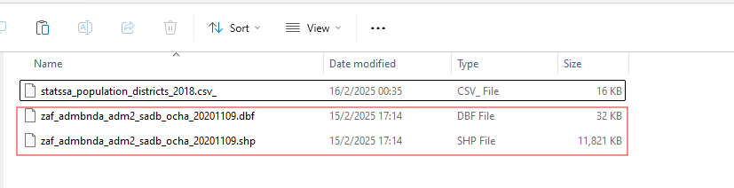
the image below is a screenshot with the relevant data needed for this presentation
Step 1
- the first thing you need is a good
base mapto work with. Depending on what you are working on , a simple map of the boundaries of SA is sufficient. - we need a shapefile to work with together with (and related files e.g dbf file that come with it as highlighted in the image above)
- The relevant command is called
shp2dtaand it creates two linked Stata files which are:- A list of all geographical units i.e for our case
SA_counties - A list of coordinates
coord_SAthat describe the related boundaries.
- A list of all geographical units i.e for our case
*****loading the shapefiles*****
shp2dta using "Datasets\zaf_admbnda_adm2_sadb_ocha_20201109", database(SA_counties) coordinates(coord_SA) genid(county_id) replace
type: 5Glimpse of the generated Datasets
use coord_SA ,clear
list in 1/5
| _ID _X _Y |
|----------------------------|
1. | 1 . . |
2. | 1 29.02187 -30.00443 |
3. | 1 29.02401 -30.00522 |
4. | 1 29.02775 -30.00661 |
5. | 1 29.02909 -30.0071 |
+----------------------------+use SA_counties ,clear
list Shape_Leng Shape_Area ADM2_ID county_id in 1/5 | Shape_~g Shape_~a ADM2_ID county~d |
|------------------------------------------|
1. | 10.01106 1.010062 DC44 1 |
2. | 5.053988 .6500897 DC25 2 |
3. | 16.2535 2.027643 DC12 3 |
4. | 8.405694 1.645116 DC37 4 |
5. | 4.47912 .2652066 BUF 5 |
+------------------------------------------+
Step 2
- we now import the Geographically disaggregated data we want to map (ie country population)
****Load stats SA population by districts for 2018*****
import delimited "Datasets\statssa_population_districts_2018.csv_", clear
rename adm2_id ADM2_ID
save "pop_districts_final.dta", replace
(encoding automatically selected: UTF-8)
(30 vars, 52 obs)
file pop_districts_final.dta savedGlimpse of the population dataset
use "pop_districts_final.dta" ,clear
list ADM2_ID p_total in 1/5
| ADM2_ID p_total |
|-------------------|
1. | BUF 834997 |
2. | CPT 4005016 |
3. | DC1 436403 |
4. | DC10 479923 |
5. | DC12 880790 |
+-------------------+
Step 3: Merge the datasets
- merge Geo-coordinates of major South African cities and Geographically disaggregated data we want to map (ie county population) > to achieve the above we need a variable that is common to both datasets and this variable is
ADM2_ID
*****Merge the datasets*********
use "SA_counties.dta", clear

merge 1:1 ADM2_ID using "pop_districts_final"
cap drop _merge

save "master_data.dta"
Result Number of obs
-----------------------------------------
Not matched 0
Matched 52 (_merge==3)
-----------------------------------------
file master_data.dta already exists
r(602);
r(602);Glimpse merged dataset (masterdata)
use "master_data.dta" ,clear
list ADM2_ID Shape_Leng Shape_Area county_id p_total in 1/5
| ADM2_ID Shape_~g Shape_~a county~d p_total |
|----------------------------------------------------|
1. | BUF 4.47912 .2652066 5 834997 |
2. | CPT 5.210914 .2383657 11 4005016 |
3. | DC1 14.65113 2.973226 48 436403 |
4. | DC10 17.86512 5.624098 6 479923 |
5. | DC12 16.2535 2.027643 3 880790 |
+----------------------------------------------------+
Step 4: Draw the map
- Having merged the county level information with master file we use the
spmapcommand to draw the map. - we specify
p_total, the variable capturing the total population in the country per Province , as the variable of interest we want to base our coloring scheme on. - we need to remind stata that the file containing the base map is called
coord_SA.dtaand the id that identifies each geographical unit is calledcounty_id - further you can add additional aesthetics to your map.
***Draw the map****

use "master_data.dta"

spmap p_total using "coord_SA.dta", id(county_id) legend(on) fcolor(Greens2) legend(label(2 "74247-502821") label(3 "502821-811400")  label(4 "811400,1164473.5" )  label(5 "31164473.5,4949347" ) ) title("Population Density by District")
 /*specify base map (coord_SA) and variable identifying relevant geographic units (county_id)*/

/*change default labels (just cosmetics really) */
quietly graph export graph_map1.svg, replace
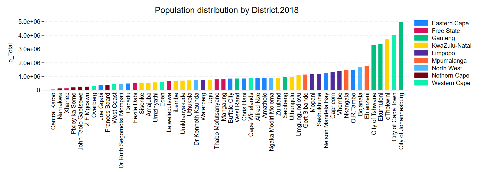
use "master_data.dta"
graph bar (asis) p_total ,title("Population distribution by District,2018") over(ADM1_EN) asyvars over(ADM2_EN , sort(p_total) lab(angle(90)))  ysize(5) nofill legend(pos(3) col(1)) xsize(14)
quietly graph export graph_1hbar.png, replace